Chapter 2 - Operators & Measurement
Reference Quantum Mechanics: A Paradigms Approach by David McIntyre.
Operators are mathematical objects that operate on kets to turn them into new kets; is one such example. If a ket is not changed by the application of some operator, then the ket is known as an eigenvector and the associated constants are eigenvalues. Above, is the eigenvector and is an eigenvalue. Both eigenvectors and eigenvalues are properties of the operator - if it changes, so does the eigenstuff. For the operator , the eigenvectors / values are:
Postulate 3: The only possible result of a measurement of an observable (like ) is one of the eigenvalues of the corresponding operator .
This postulate implies that, if we have the eigenvectors and values of , we can actually reconstruct from them.
Let . Which leads us to Now, plugging these solved values in,
- Operators are diagonal in their own basis (i.e. they only have elements along the main diagonal).
- The elements along the diagonal are the eigenvalues of the operator.
- The eigenvectors themselves are not included in the operator matrix.
Note: an observable is some physical quantity that can be measured - such as spin. In that context, the operator represents that observable.
Other representations of matrix elements
We can also represent an operator matrix in terms of its elements. Let the operator describe some two-dimensional spin-1/2 system (like does).
Where
Finding eigenvectors / values from an observable
If we know the operator , and need to find the possible results of a measurement of the corresponding observable, we can start from the general eigenvalue equation and work from there.
where is the eigenvalue and is the corresponding eigenvector. Eigenvalues can be found then by solving the secular equation, Note: for a operator (i.e. a spin-1/2 system), this is .
After finding the eigenvalues, we now know and - all that remains is to find by solving for it in .
The process of finding the eigenvectors and eigenvalues of a matrix is known as diagonalization.
Hermitian operators
To find the associated bra operator to some operator acting on a ket, we use the operator
where is the Hermitian adjoint of , found by transposing and taking the complex conjugate of . If , then is said to be Hermitian, and for .
This is not normally the case - if is not Hermitian, the corresponding bra-state operator will be different from - i.e. will not be the bra corresponding to .
Hermitian operators have some properties to be aware of:
- They will always have real eigenvalues which ensures the results from a measurement are always real.
- The eigenvectors of a Hermitian operator form a complete set of basis states, ensuring we can use the eigenvectors of any observable as a valid basis.
New operators
Let's say we wanted to find the spin component in some general direction .
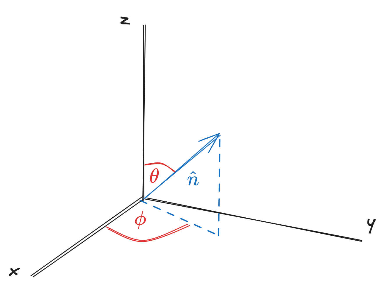 where . Projecting the spin vector onto such that
then
and diagonalizing the vector above, we find the eigenvectors for to be
with the state vector
where . Projecting the spin vector onto such that
then
and diagonalizing the vector above, we find the eigenvectors for to be
with the state vector
Note: the coefficient calculation attached to is from total probability being equal to 1.
Outer product
Instead of taking the inner product between two state vectors, we can also find the outer product (). For example, we can rewrite as and are called projection operators:
This last formula is known as a closure or completeness relation due to the equivalency to the identity operator , meaning that these basis states form a complete set of states.
When our projection operator acts on some state ,
Note: is equivalently the or coefficients.
and the probability of observing some state is then This allows us to write the fifth postulate
Postulate 5: After a measurement of some observable operator that yields the result , the quantum system is in a new state that is the normalized projection of the original system ket onto the new ket corresponding to the result of the measurement
Returning to Stern-Gerlach 3 & 4
We were able to look at experiments 1 and partially 2 in chapter 1, but not experiments 3 and 4, which required expounding on operator products a bit further.
Experiment 3
Experiment 3 measured , then measured , then again, observing a "reset" with the other measurement.

The probability that an atom stays throughout the three measurements is the product of each probability - such that
Likewise for it to be , then , then is
Tradition holds QM magnitudes / probabilities to be read from right to left.
Experiment 4
Experiment 4 measured , then put the atoms through an analyzer (but didn't measure them), then measured again, finding the "measurement" step to be an important one.
 The results in this one are interesting but simple - representing them with postulate 5,
This can be expanded out (and is done so in McIntyre 2.2.4), but will not be included here for the sake of brevity.
Mean and Standard Deviation
The expected mean (or expectation value) of some measurement is represented by , such that and is a sum of each possible result multiplied by the probability of that result.
Probability can be represented by both outer products and inner products - inner products are more readable, but require squared absvals , while outer products require more terms overall.
We can also write the expectation value for some operator as For , this can be written out as
Which makes sense, given is the only possible result of a measurement of for the state. For some system prepared .
Standard Deviation
The root-mean-square deviation (r.m.s. deviation) is
In the rightmost version, the second term is the squared expectation value. The first term, in the case of the initial state, can be expanded into and Expected, since we only have one possible result for measuring - so no spread of possible results.
Commuting Observables
Note: eigenstates are equivalent to eigenvectors.
The commutator for two operators is defined as If the commutator is zero, then the two operators (observables) commute. If nonzero, they don't commute. Logical consequences can be determined by just this statement alone - the first being: The order of operation doesn't matter for commuting observables. Now, let be an eigenstate (eigenvector) for some operator with eigenvalue : Let's apply to both sides of this. Using the commutability of and , This last equation says is also an eigenvector of corresponding to the same eigenvalue . Thus, must be a scalar multiple of (let's say this scalar multiple is ) - and we can write Commuting operators will therefore share common eigenvectors - this means the two operators (that represent observables) are compatible, and we can measure one without erasing our knowledge of the results of the other observable.
This is often phrased as knowing the results of these observables simultaneously, though realistically we're still measuring each sequentially.
If two operators do not commute, then they are incompatible. This is the case for our orthogonal spin operators - and the commutations for , and are
The Uncertainty Principle
We can relate the product of two standard deviations (i.e. uncertainties) of two observables with the commutator by
The Uncertainty Principle: the product of two uncertainties will always be greater than or equal to the absolute expected value of the two.
For the and spin components,
Implying and - while we can know one spin component, we can never know the other two (they are incompatible observables).
Operator
and is represented in matrix form as
Thus, since the operator is proportional to the identity operator, it must therefore commute with all the other operators and - this implies all states are eigenstates of the operator, and we can write for any state in the spin-1/2 system. The vector has an expectation value of
and a "length" of
This is longer than the "normal" measured component of along any axis - implying the spin vector can never be fully aligned along any one axis, since there will be always components in other axes.
This is often called "quantum fuzziness".
Regarding Photons
Photons also have spin - but due to moving at (ultra-relativistic), it can never have a spin of 0 - must be either .
Spin-1 Systems
Fermions are particles with spins of multiples of 1/2 (i.e. , , ), while bosons are those with full-integer spins (i.e. , , ). Spin-1 bosons have spin states of , or
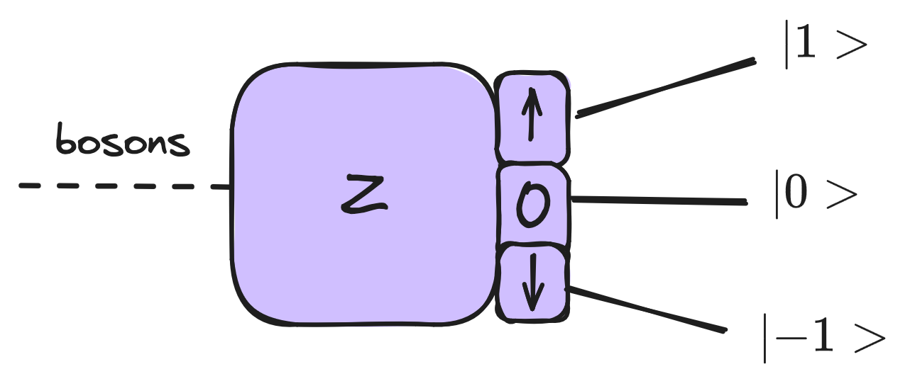 where
where
The eigenvalues , and are on the main diagonal of .
For ,
and for ,
Note: The Stern-Gerlach experiments have conceptually the same results - but note that experiment 2 differs (not all 1/3 - rather, one is 1/2, the other two 1/4).
General Quantum Systems
Let denote the spin of some -spin system with number of beams (i.e. for a spin-1 system, this would be 3, spin-1/2 system, 2). Let the possible values for spin on the axis be labeled by - then,
is known as the spin (angular momentum) quantum number and is the spin component quantum number (or magnetic quantum number).
In spin-1/2, and in spin-1,