Useful stuff
Here I'm putting useful commands, dotfiles and links to remember.
Links
I love:
Commands
To convert a bunch of images from one format to another via ImageMagick
mogrify -format jpg *.heic
To convert some audio files from one sample/depth to another via sox
mkdir converted; for flac in *.[Ff][Ll][Aa][Cc]; do sox -S "$flac" -R -G -b 16 converted/"$flac" rate -v -L 44100 dither; done
To enable scientific notation in qalc
set exp # set exp 0 to disable
Dotfiles
Alacritty
Located at ~/.config/alacritty/alacritty.toml.
[env]
TERM = "xterm-256color"

[window]
opacity = 0.8
blur = true

[window.dimensions]
columns=100
lines=30

[font]
normal.family = "MesloLGS NF"
size = 12
Last command in Fish (!!)
Put in ~/.config/fish/config.fish.
function last_history_item; echo $history[1]; end
abbr -a !! --position anywhere --function last_history_item
Using the PIC16F88 as an I2C device
Final project for PHYS 335A: Digital Electronics, taught Spring of 2024 by Dr. David Pengra at the University of Washington.
The PIC16F88 is a 16-bit, lightweight microcontroller from Microchip devices which is useful for a variety of low-cost and low-power, high speed embedded systems operations.
Here I describe some details of how I try to set up an IC implementation on the PIC16F88, and design a program using MPASM Assembly language to operate it as an I2C target device (slave), to be controlled by higher-level controller (master) devices such as Arduinos or Raspberry Pis.
Note: MPASMx is no longer supported as of MPLAB X v5.40 - use >v5.35 if you're intending to use it here. See the footnote1 for more details on this & using OSx.
Introduction to I2C
IC (or inter-integrated circuit) is, like so many things in electrical engineering, a complicated-looking protocol that's actually pretty simple in a clever sort of way.
When compared to its closest serial communications cousin SPI (or serial peripheral interface), IC only requires 2 datalines (SDA and SCL) compared to SPI's 4 (MISO, MOSI, SCLK and CS), and allows for far more devices to be connected due to the use of peripheral addressing rather than SPI's chip select.
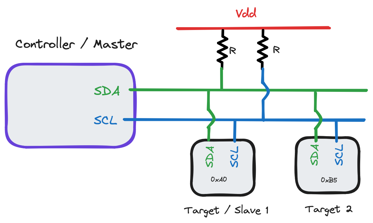 The master device / controller, in my case an Arduino Mega 2560, specifies some baudrate to operate the clock frequency on. When no data transmission is happening, both SDA and SCL are pulled to
 Vdd through the pullup resistors ( above - typical choices range from
4.7k to 10k).
Since this implementation of IC is open-drain, the controller and target oscillate lines by just directly grounding them - the pullup resistors avoid shorting the circuit out this way. Note this means that the longer SCL=0 or SDA=0, the more power the circuit will use by extension.
Pullup resistor choice is important if you're trying to optimize - small PU resistors have high power consumption but also high speeds, while large PU resistors have low power consumption but also create capacitance delays. Texas Instruments has a good description of this.
By my understanding, IC (in 7-bit addressing space2) generally operates like this:
- Controller device sends a
STARTbit by holding SDA low with SCL high. - Controller sends a 7-bit address, one bit per clock cycle.
- At the 8th bit (8th time SDA goes HIGH), target devices compare the sent address with their own. If the two match, continue. Otherwise, ignore - this stream isn't meant for that device.
- Controller and specified target communicate.
ENDbit set by either to indicate the conversation ifs over.
Each 'communication sequence' happens in 8-bit intervals - 7 bits for data, the 8th allowing time for each device to tell the other what to expect next. The PIC16F88 SSP section of the datasheet has a handy visualization of the target transmitting data back to the host - what we're planning on doing here.
![]()
So - let's talk about the project.
I2C Rangefinder Project
We'll use the PIC16F88 in conjunction with the HC-SR04 ultrasonic rangefinder module to create a rangefinding device, retrieving the rangefinder values from the PIC by communicating over IC.
For our controller, we'll use an Arduino Mega 2560 - chosen because it allows serial console monitoring & has 5V IC logic by default (the PIC16F88 uses 5V, and thus has 5V IC outputs), and has a number of high-level logic libraries for interfacing with IC (see the Wire library for more information).
It is possible to use an IC controller with 3.3V logic (such as a Raspberry Pi) with 5V target devices or visa-versa, however you'll need to convert logic levels between the two, either with a dedicated logic-level conversion device or by using N-channel MOSFETs and pull-up resistors. Refer to NXP note AN10441 for more information.
Hardware
Making a circuit diagram for this,
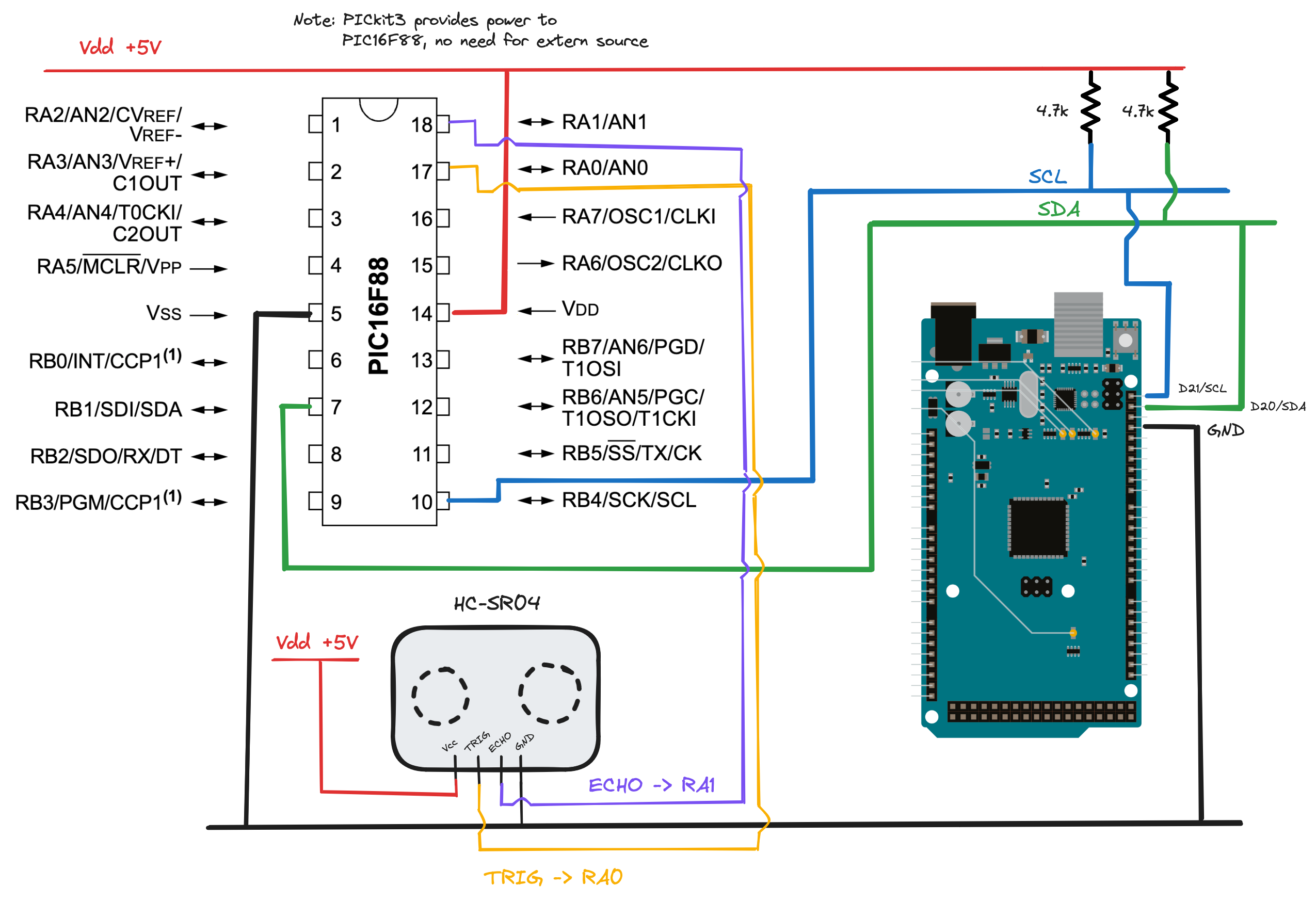 For my pullup resistors I decided to use 4.7k, as I'm not particularly worried about power consumption on a proof-of-concept. Note that
 RA<x> refers to pins PORTA<x>, and similarly RB<x> refer to pins PORTB<x>.
Note: it's quite important that the controller and target devices share a common ground - otherwise, the "reference ground voltage" for IC pulses may not be the same and a circuit may not function as hoped!
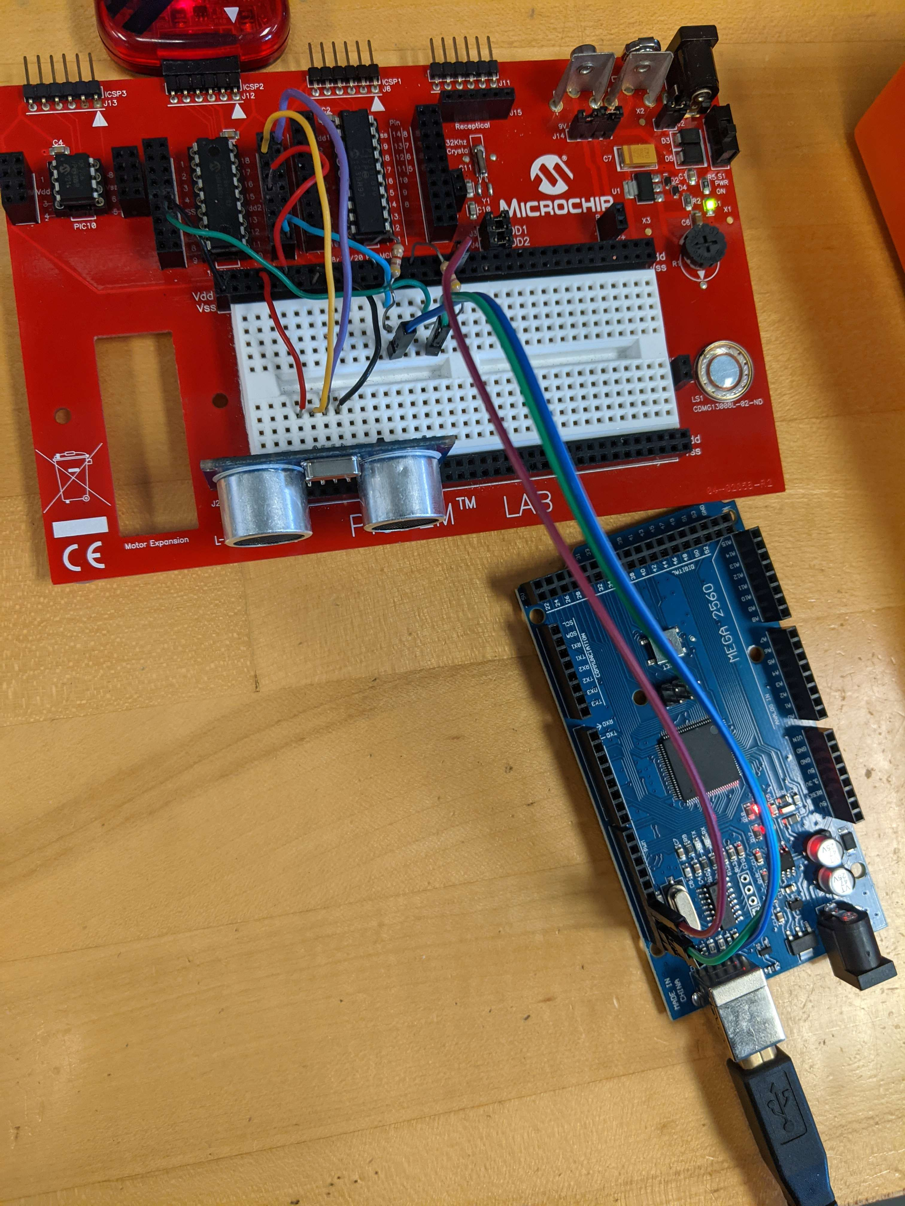
Here's the physical implementation of this circuit.
Software
First, I made sure code for the rangefinder was working before fiddling with IC. I made use of some of the code provided in Lab 8 - Sonic Ranger with Interrupts & Hardware Control, ensuring the rangefinder worked by tinkering with the debugger and observing variable changes in response to changed echo distances from the rangefinder. This could have also been done by reusing our Lab 7 code, but I thought the Lab 8 code looked much neater.
Now - onto the software side of IC. The SSP section on IC in the PIC16F88 datasheet is unfortunately quite lacking with regards to exact implementation methods, so I was forced to scrounge around a bit through sources official and otherwise for information.
In brief, the PIC16F88 doesn't easily support a controller-mode implementation of IC out of the box, lacking the MSSP register found in other PICs that would allow easier implementation.
Instead, the 'F88 supports a variety of both SPI and IC target device implementations that may be used instead - refer to Register 10.2 in the datasheet SSP section. If you're looking to implement master-mode on a PIC, look to other devices such as the PIC16F1508 which have MSSP registers.
Using the PIC16F88 datasheet section on SSP (paying particular attention to section 10.3.1) as well as the section on interrupts and the section on configuring PORTB, here's the process I followed to implement "IC Slave mode, 7-bit address with Start and Stop bit interrupts enabled".
- Clear
ANSELto enable digital (instead of analog) inputs. - Set
TRISB<1>(SDA) andTRISB<4>(SCL) pins, turning them into inputs.- "But wait! IC is bidirectional!" you might argue - this is true. The SSP (synchronous serial port) module in the PIC16F88 will automatically set and clear
TRISB<1>/<4>in response toSDAandSCLevents.
- "But wait! IC is bidirectional!" you might argue - this is true. The SSP (synchronous serial port) module in the PIC16F88 will automatically set and clear
- Set bits in
SSPCON(SSP control register):SSPCON<5>-SSPEN, enables SSPSSPCON<4>-CKP, clock polarity, allowing controller to oscillateSCLSSPCON<3:0>=1110-SSPM<3:0>, "SSP mode select". See Register 10.2 in the SSP section of the datasheet for other options - by using1110, we're setting our SSP mode to IC target mode with 7 bit addressing, start/stop interrupts enabled.
- Choose an address for your device. It must not be
0x00or0x01, other values allowed up to0xFF. I chose0x77arbitarily. Write it intoSSPADD.- Since only bits
SSPSR<7:1>are compared toSSPADD, run anRLFinstruction (rotate-left-through-carry) onSSPADDto make sure your address matches the checked one.
- Since only bits
- Enable interrupts. Set bits:
INTCON<7>-GIE, enable global interruptsINTCON<6>-PEIE, enable peripheral interruptsPIE1<3>-SSPIE, enable SSP interrupts
- Create interrupt functions in your ISR space
- Check if
PIR<3>(SSPIF) is set to make sure the interrupt was caused by IC, if there are multiple possible interrupts in your code. - Function to
SaveSTATUSandWas you normally would. WriteData- to send data, write (less than 8 bits total) toSSPBUF, then setSSPCON<4>to indicate to the controller that you (the target) are ready to transmit.SSPBUFwill now start automatically sending.- Function to
Loadas you normally would - Clear
PIR1<3>(SSPIF) to reset the SSP ...
- Check if
- ... and
RETFIE.
My ISR implementation following 6-7 above looks like this:
; Interrupt Service Routine ----------------------------------------------------

	ORG 0x0004 ; ISR beginning

SaveState
	MOVWF SAVE_W ; Save W register
	SWAPF STATUS, W ; Save STATUS reg
	MOVWF SAVE_STAT ; ... into temporary reg

LoadAndSend
	MOVFW TimerCounts ; Load last pulse period into W
	MOVWF SSPBUF ; Load SSPBUF with W (will be sent)
	BSF SSPCON,CKP ; Set CKP bit to indicate our buffer is ready

LoadState
	SWAPF SAVE_STAT,W ; Load STATUS
	MOVWF STATUS
	SWAPF SAVE_W, F ; Load W
	SWAPF SAVE_W, W ; Load W into W

	BCF PIR1,SSPIF ; Clear serial interrupt flag
	RETFIE ; ... and return to program execution

; End ISR ----------------------------------------------------------------------
and relevant IC code blocks like this:
; I2C initialization subroutine ------------------------------------------------

SetI2C
    BANKSEL	ANSEL           ; Bank 1
    CLRF	ANSEL           ; Set to all-digital inputs
    BSF		TRISB, TRISB1	; Set PORTB<1> (SDA) as an input
    BSF		TRISB, TRISB4	; Set PORTB<4> (SCL) as an input
    CLRF	SSPSTAT		; Reset SSPSTAT

    BANKSEL	SSPCON		; Bank 0
    BSF		SSPCON, SSPEN	; Turn on SSP
    BSF		SSPCON, CKP	; Enable clock (if 0, holds clock low)
    BSF		SSPCON, SSPM3	; I2C 7-bit slave-mode w/ int is SSPM<3:0>=1110
    BSF		SSPCON, SSPM2
    BSF		SSPCON, SSPM1
    BCF		SSPCON, SSPM0

    BANKSEL	SSPADD		; Bank 1
    MOVLW	I2C_ADDR	; Load I2C address into W
    MOVWF	SSPADD		; Load SSPADD with I2C_ADDR (0xIC random)
    RLF		SSPADD,F	; Left-shift since SSPSR<7:1> compared

    ; Interrupt configuration
    BANKSEL	INTCON		; Bank 0
    BSF		INTCON, GIE	; Enable global interrupts - SSP interrupt on START
    BSF		INTCON, PEIE	; Enable peripheral interrupts
    BANKSEL	PIE1		; Select PIE register
    BSF		PIE1, SSPIE	; Enable SSP interrupts in peripheral interrupt reg

; End subroutine ---------------------------------------------------------------
Results
Using the Arduino IDE with the Wire library, I set up a basic script that, after initializing IC and the serial monitor both at a baudrate of 9600, would send an IC "read" query down SDA to address 0x77 (our PIC) to try and retrieve our TimerCounts value from our interrupt function LoadAndSend shown above.
#include <Wire.h>

// Notes: D21 is SCL, D20 is SDA for MEGA 2560

void setup() {
  // Initialize I2C
  Wire.begin();

  // Start serial output for console monitoring
  Serial.begin(9600);
  Serial.println("Setup complete. Starting loop ...");
}

// Poll 0x77 address - then sleep for two seconds - then poll.
void loop() {
  // Request 2 bits from 0x77
  Wire.requestFrom(0x77, 1);

  // Send results (if any) to serial monitor
  while (Wire.available()) {
    char c = Wire.read();
    Serial.print("Distance: ");
    Serial.print(c, DEC);
    Serial.println(" cm");
  }

  delay(2000);
}
And, after some tinkering, checking the serial monitor revealed ...
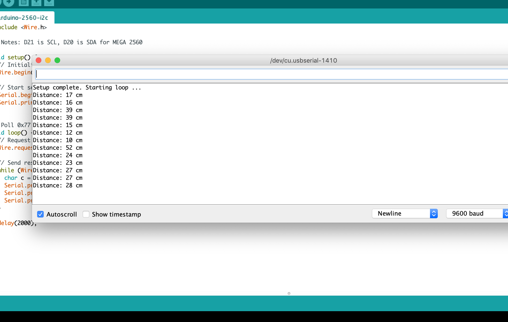
Voilà!!
Notes
I definitely didn't get this first try - I wrote the Arduino script pretty early on to monitor the PIC16F88 while I figured out the maze of interrupt flags necessary to work with IC.
Something I should note - I've wasted at least a few hours during this project because I wasn't operating on the correct bank while trying to operate on some register. Such problems won't often be immediately apparent, only becoming clear when you step through your code with a debugger and realize a value isn't changing when it should.
BANKSELis a friend!
Code
The full program I used for this is written below.
;*******************************************************************************
;
;    Filename: Final Project I2C Ranger
;    Date: 5/31/2024
;    File Version: 1.0
;    Author: Parker Lamb
;    Description: Sets PIC16F88 up as I2C-ready ultrasonic rangefinding device.
;
;*******************************************************************************

;*******************************************************************************
;
;                Procesor initial setup
;
;*******************************************************************************

    list       F=inhx8m, P=16F88, R=hex, N=0 ; File format, chip, and default radix

#include p16f88.inc ;   PIC 16f88 specific register definitions

    __config _CONFIG1, _MCLR_ON & _FOSC_INTOSCCLK & _WDT_OFF & _LVP_OFF & _PWRTE_OFF & _BODEN_ON & _LVP_OFF & _CPD_OFF & _WRT_PROTECT_OFF & _CCP1_RB0 & _CP_OFF
    __config _CONFIG2 , _IESO_OFF & _FCMEN_OFF

    Errorlevel -302 ; switches off msg [302]: Register in operand not in bank 0.

;*******************************************************************************
;
;                Constants and variables
;
;*******************************************************************************

; Program vars
TimerCounts EQU     h'20'	; Saving timer counts

;  vars
SAVE_W	    EQU	    h'21'	; Interrupt temporary W storage
SAVE_STAT   EQU	    h'22'	; Interrupt temporary STATUS FSR storage

; I2C status
I2C_STAT    EQU	    h'23'	; Check if I2C is connected
I2C_ADDR    EQU	    0x77	; I2C address (const)

; Delay count registers
DInd1	    EQU	    h'24'
DInd2	    EQU	    h'25'

; Delay times
DTime1	    EQU	    .199	; 60 ms delay - outer loop
DTime2	    EQU	    .60		; Nested loop runs for 59,941 cycles

; SCL and SDA locations
#define	    _SDA    PORTB,RB1	; Make _SDA easier to check
#define	    _SCL    PORTB,RB4	; Make _SCL easier to check

;*******************************************************************************
;
;                Memory init & interrupts
;
;*******************************************************************************

	    ORG	    0x00
	    GOTO    Init

; Interrupt Service Routine ----------------------------------------------------
            ORG     0x0004               ; ISR beginning

SaveState
    MOVWF	SAVE_W		; Save W register
    SWAPF	STATUS, W	; Save STATUS reg
    MOVWF	SAVE_STAT	; ... into temporary reg

LoadAndSend
    MOVFW	TimerCounts	; Load last pulse period into W
    MOVWF	SSPBUF		; Load SSPBUF with W (will be sent)
    BSF		SSPCON,CKP	; Set CKP bit to indicate our buffer is ready

LoadState
    SWAPF	SAVE_STAT,W	; Load STATUS
    MOVWF	STATUS
    SWAPF	SAVE_W, F	; Load W
    SWAPF	SAVE_W, W	; Load W into W

    BCF		PIR1,SSPIF
    RETFIE			; ... and return to program execution

;*******************************************************************************
;
;                Program start
;
;*******************************************************************************
Init	    ORG	    0x0020

; Set up oscillator to 4 MHz
SetOsc_4MHz
    BANKSEL	OSCCON
    CLRF	OSCCON
    BSF		OSCCON, IRCF1   ; Bit 5
    BSF		OSCCON, IRCF2   ; Bit 6

    ; Tuned value from Lab 7 - adjust as needed
    MOVLW	0x16
    MOVWF	OSCTUNE

; Reset IO to all digital, all outputs, clear latches
ResetIO
    BANKSEL	PORTA   ; Clear data latch registers
    CLRF	PORTA
    CLRF	PORTB
    BANKSEL	TRISA   ; Data direction on PORTA / PORTB
    CLRF	TRISA   ; Set PORTA to all output
    CLRF	TRISB   ; Set PORTB to all output
    BANKSEL	ANSEL   ; Select digital / analogue register
    CLRF	ANSEL   ; And set to all-digital inputs

; ... and set what we need to
SetIO
    BANKSEL	TRISA
    MOVLW	0xFF
    MOVWF	TRISA		; Set PORTA direction to all inputs
    BCF		TRISA, RA0	; ... except PORTA<0>, an output

SetTMR0
    ; TMR0 duration between pulses indicates our radar distance
    BANKSEL	OPTION_REG	; TMR0 operation controlled via OPTION_REG
    CLRF	OPTION_REG	; Clear it - sets PSA to TMR0, low-hi edge
    BSF		OPTION_REG, 0x0
    BSF		OPTION_REG, 0x2	; Set prescaler rate to 1:64 w.r.t oscillator (101)
    BANKSEL	INTCON		; Select interrupt control register
    BCF		INTCON,TMR0IE	; Disable TMR0 OF interrupt (not using here)
    BCF		INTCON,TMR0IF	; Clear flag (maybe unnecessary - do anyway)

;*******************************************************************************
;
;                I2C configuration
;   We're using this device in 7-bit I2C slave-mode with stop + start
;   interrupts enabled.
;
;*******************************************************************************

SetI2C
    BANKSEL	TRISB		; Bank 1
    BSF		TRISB, TRISB1	; Set PORTB<1> (SDA) as an input
    BSF		TRISB, TRISB4	; Set PORTB<4> (SCL) as an input

;    BANKSEL	SSPSTAT		; Bank 1
    CLRF	SSPSTAT		; Reset SSPSTAT

    BANKSEL	SSPCON		; Bank 0
    BSF		SSPCON, SSPEN	; Turn on SSP
    BSF		SSPCON, CKP	    ; Enable clock (if 0, holds clock low)
    BSF		SSPCON, SSPM3	; I2C 7-bit slave-mode w/ int is SSPM<3:0>=1110
    BSF		SSPCON, SSPM2
    BSF		SSPCON, SSPM1
    BCF		SSPCON, SSPM0

    BANKSEL	SSPADD		; Bank 1
    MOVLW	I2C_ADDR	; Load I2C address into W
    MOVWF	SSPADD		; Load SSPADD with I2C_ADDR (0xIC random)
    RLF		SSPADD,F	; Left-shift since SSPSR<7:1> compared

    ; Interrupt configuration
    BANKSEL	INTCON		; Bank 0
    BSF		INTCON, GIE	; Enable global interrupts - SSP interrupt on START
    BSF		INTCON, PEIE	; Enable peripheral interrupts
    BANKSEL	PIE1		; Select PIE register
    BSF		PIE1, SSPIE	; Enable SSP interrupts in peripheral interrupt reg

;*******************************************************************************
;
;                Main program loop
;   Cause the sonic module to pulse every 10 microseconds. Wait for a response,
;   then save time it took into a register. Repeatedly do this.
;
;   Once I2C interrupt is detected, send information via I2C.
;
;   TODO only start this loop if START condition detected, stop with I2C STOP.
;
;*******************************************************************************
    ; Reset to bank 0
    BCF	    STATUS, RP0
    BCF	    STATUS, RP1	    ; All of the action is in Bank 0 now

MainLoop
; Send sonic device a 10-microsecond pulse
Pulse
    BSF		PORTA, RA0	; Set PORTA<0> output to high
    NOP
    NOP
    NOP
    NOP
    NOP
    NOP
    NOP
    NOP
    NOP
    BCF		PORTA, RA0	; Set PORTA<0> output low

; Loop until PORTA<1> goes HI, indicating a response
WaitForResp
    BTFSS	PORTA, RA1	; Check PORTA<1>
    GOTO	WaitForResp	; ... and loop if it's still zero

    ; Start of our response
    CLRF	TMR0		; Start timer from now
WaitUntilLow
    BTFSC	PORTA, RA1	; Check PORTA<1> to see if response finished
    GOTO	WaitUntilLow	; ... loop if still not LOW

    ; We have a response! Store timer value in a variable
    MOVFW	TMR0
    MOVWF	TimerCounts

    ; Delay for a bit so we aren't constantly polling
    CALL	Delay

    ; Return to MainLoop
    GOTO	MainLoop

;*******************************************************************************
;
;                Subroutines
;
;*******************************************************************************
; Loop from Template_for_Ranger_with_interrupts.asm, course lab template
Delay
		MOVLW   DTime2
		MOVWF   DInd2
Loop1		MOVLW   DTime1
		MOVWF   DInd1
Subloop1	NOP
		NOP
		DECFSZ  DInd1,F
		GOTO    Subloop1
		DECFSZ  DInd2,F
		GOTO    Loop1
	RETURN

Finish
    END
The code for the Mega 2560 is written in Results.
-
With version v5.40 of MPLAB X, Microchip's dedicated compiler/IDE, Microchip upgraded all their binaries to 64-bit. However, since
mpasmxwas not updated from 32 bits, and Mac OSx does not support 32-bit applications since Mojave, Mac users will need to either use Windows or a VM. ↩ -
See Wikipedia's page for addressing structure for more details. ↩
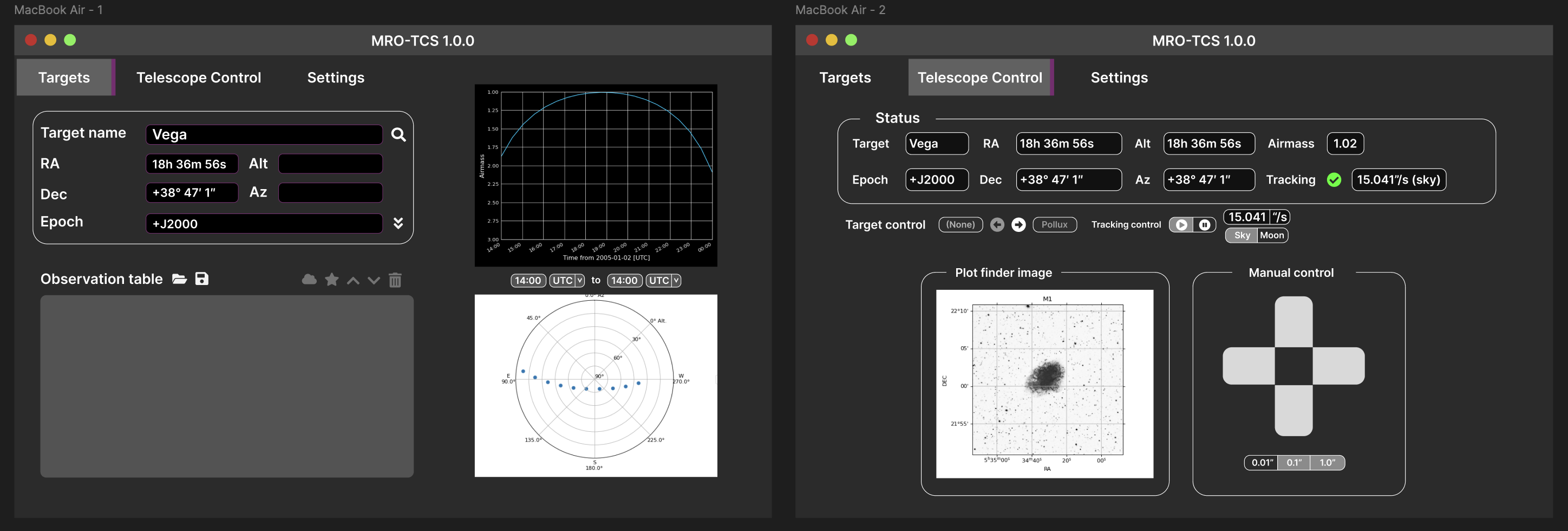
Building an ASCOM frontend for the MRO
As part of one of my final projects with the UW AUEG, this post covers the construction of a custom frontend interface to interact with the new Sidereal Technology ForceOne (F1) telescope controller we're installing April-June 2025.
Many of the telescope systems within the UW Manastash Ridge Observatory haven't been updated in a while, with 'a while' meaning (in the 21st century) to (ever). Given the telescope was originally built in 1975, that means many of the systems and electronics are ancient, creaky and sometimes just plain don't work.
One of those systems in the 'ever' category is the old telescope control system, which controls the telescope mount and helps tell it where to point - quite a critical system. Alas, like a cranky child, it's one that is prone to issues, needs constant monitoring and wire-jiggling, and just generally can be a headache sometimes.
So, after summoning our inner crusty old engineers and putting on some gloves, we've decided to rip out everything and replace it with ✨ better stuff ✨.

The Promised Land a.k.a. the ForceOne Brushless Controller uses a protocol called ASCOM ("Astronomy Common Object Model") which is a standardized set of instructions that we can use to communicate with motorized telescope mounts.
ASCOM1 is really just a set of standards for communicating with a telescope - it's like the metric measuring system, or Python's PEP8 style guide. It covers most of the use cases for interacting with a telescope, including focusing, GOTO, dome controls, filter wheels, even safety monitoring.
We're only focusing on one subset of these commands: those that can be used to control the telescope mount.

There are some pre-existing GUIs and frontends for working with ASCOM, but I didn't like any of them and some of them were expensive so we decided to make our own.
In all seriousness, most existing GUIs are designed around general use cases for ASCOM, and either have too many options for our limited use, or too few. By making our own user interface, we can make something for our own use case, and just for it.
Design and implementation
Generating a mockup for such a frontend in Figma as a way to guide development:
-
ASCOM is cool. If you're a nerd like me and love cool APIs, see the ASCOM API which is a comprehensive set of HTTP API endpoints that are broadcast by the controller (the F1 in our case) and are how we communicate with the telescope base. ↩
Internal Combustion Engines
Notes and links regarding the history and design of internal combustion engines (such as diesel and gasoline engines).
Resources:
- Wikipedia: Internal Combustion Engine
- Wikipedia: Diesel engine
- Wikipedia: Petrol engine
- Wikipedia: Engine efficiency
Questions:
- Air-alone combustion engine?
- History?
- Energy requirements of gasoline and diesel (and ethanol and natural gas)
- Ideal gas law, assuming the same combustion chamber size
- How much energy per cycle? Exhaust per cycle?
- Chemical reaction of diesel and normal gas
Fundamentals
There are two main types of engines:
- Internal combustion engines (i.e. gasoline, diesel, turbine)
- External combustion engines (steam piston, steam turbine, Stirling engine)
- Uses some working fluid, incl. air, steam or pressurized water.
Every engine has something called an 'efficiency' associated with it. The thermodynamic definition of it is:
is the heat absorbed by the process, and is the work done on the driveshaft (useable energy delivered). 100% efficiency would use all heat, which is the result of the combustion reaction.
In a practical sense, efficiency details how much energy is lost to mechanical processes, such as thermal expansion and friction.
On a fundamental level: internal combustion engines are heat engines which use the energy released in a combustion reaction (some fuel, like coal gas, with some oxidizer like air) to do work on mechanical components (like pistons), such that:
- Fuel and air enter a combustion chamber,
- are (usually) then compressed by some piston,
- which increases the pressure and temperature of the mixture,
- which is then ignited (either via pressure alone or by a spark),
- causing a combustion reaction, which releases heat, light and exhaust,
- driving the piston back up,
- which converts thermal into kinetic energy,
... which then can be used to drive some external mechanical device, like a vehicle crankshaft or drive system.
Further, there are two primary types of combustion ignition in both ICE and ECE:
- Intermittent combustion, where combustion might happen once every few "strokes" (two, four, six stroke engines).
- Continuous combustion (like rockets, jet engines and turbine engines).
Brief bit of history
The first "recognizable" form of an internal combustion engine emerged as early as the 12th century in China in a very different form: the cannon.

Gunpowder is a mixture of charcoal (15%), sulfur (10%) and saltpeter (potassium nitrate), (75%). The former two form the fuel, while the latter is the oxidizer1.
When a spark is put to the mixture, the oxygen contained within the potassium nitrate reacts with the sulfur and charcoal in the reaction described above. As the reaction exhaust gasses are created, they put mechanical force on the cannonball, converting the chemical potential energy to kinetic energy on the cannonball.
It was inefficient though - under completely ideal circumstances, we might expect an efficiency around ~30%2 (i.e. 30% of the chemical potential energy is converted to kinetic energy of the projectile), with real-world scenarios demonstrating significantly lower efficiency (15-25%).
The remaining energy might go into heating the exhaust gasses (~35%), the heat of the combustion chamber (~30%), friction of the ball leaving the cannon (basically heating the chamber as well, ~2%) or as still unburned propellant (if the mixture was not completely proportional).
Cannons are, however, relatively single-use compared to reciprocating engines. Once the ball left the chamber, the "combustion chamber" ceases to exist until a new ball is loaded.
Gas engines
Various patents existed for liquid and gas engines starting in the late 18th century, including the Barber gas turbine (1791), the Street liquid gas engine (1794), and the Niépce brothers' internal combustion engine (1807), which ran on a dust mixture and powered a boat (granted a patent by Napoleon).
In 1860, Étienne Lenoir (a Belgian engineer) invented (and actually made) the Lenoir engine, which used both coal gas and air. It was not the first ever to be made (De Rivaz designed, in 1808, "the world's first internal combustion powered automobile"), but it was the first to be both produced in quantity, and be able to be used in practical scenarios (test drive from Paris to Joinville-le-Point, 18 km in 3 hours, so about 6 km/h).
(image of it here)
The engine was, however, quite inefficient (~1.2-5.4 m/kWh), loud, and overheated easily.
Continued gas engine development
The Lenoir engine provided the framework by which most internal combustion engines would continue to emerge through the 19th and 20th centuries, including:
- 1864, Nicolas Otto invented the first atmospheric gas engine.
- 1872, George Brayton created the first commercial liquid ICE.
- 1876, Otto worked with Gottlieb Daimler and Wilhelm Maybach to create a compressed-charge four-stroke engine.
- 1879, Karl Benz created a reliable two-stroke engine, and began production on commercial vehicles using it and a later four-stroke engine (most 3-wheel).
- 1892, Rudolf Diesel developed the first compressed-charge, compression ignition engine.
Engine types
There are two primary types of engine: intermittent, and continuous. Subdividing each:
Intermittent
Modern intermittent engines include primarily reciprocating engines and rotary engines.
Reciprocating engines:
- Two-stroke: one cycle per crankshaft rotation.
- Four-stroke: four separate steps, occurring in two cycles. s
Sources
-
https://www.usni.org/magazines/proceedings/1879/december/chemical-theory-combustion-gunpowder ↩
-
https://en.wikipedia.org/wiki/Physics_of_firearms ↩
Chapter 1 - Relevant Mathematics
Reference "Introduction to Electrodynamics" by David Griffiths.
Vectors
We start with a brief review of vector algebra - I'll skip most of it but keep the key things.
Dot product
The dot product is a measure of how "parallel" two vectors are, maximized when parallel, minimized (0) when perpendicular.
It is commutative () and distributive (). The result of the dot product is a scalar.
Cross product
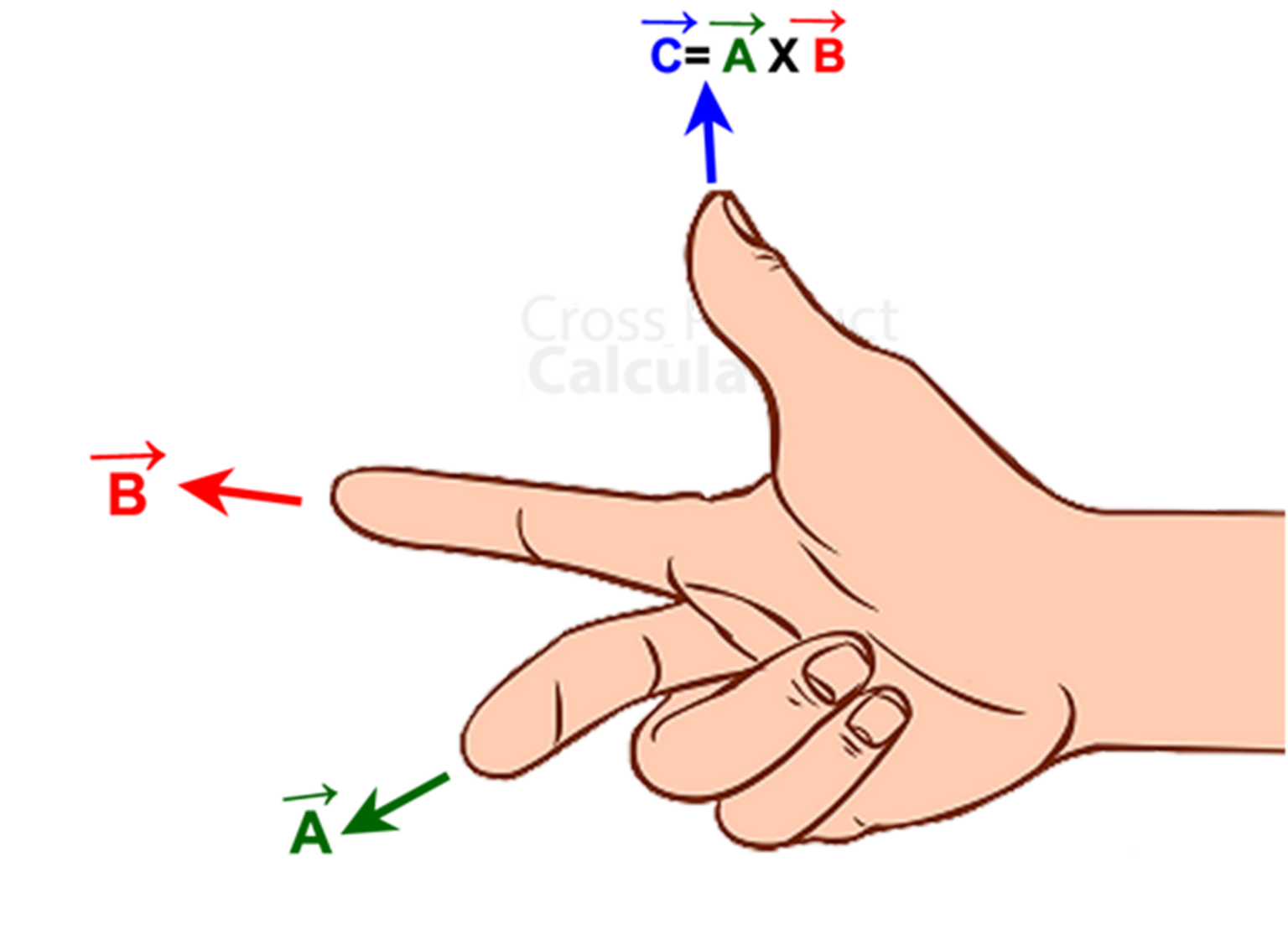
The cross product yields a third vector orthogonal to both and , maximized in magnitude when and are themselves orthogonal to one another.
 The cross product is distributive, but not exactly commutative - instead,
Some other properties:
The cross product is distributive, but not exactly commutative - instead,
Some other properties:
- The result of the cross product is a vector, not a scalar.
- The magnitude of the cross product is the area of the parallelogram generated by and .
- The cross product of a vector with itself is zero.
We can calculate a cross product like so:
where is the normal to the plane formed by and .
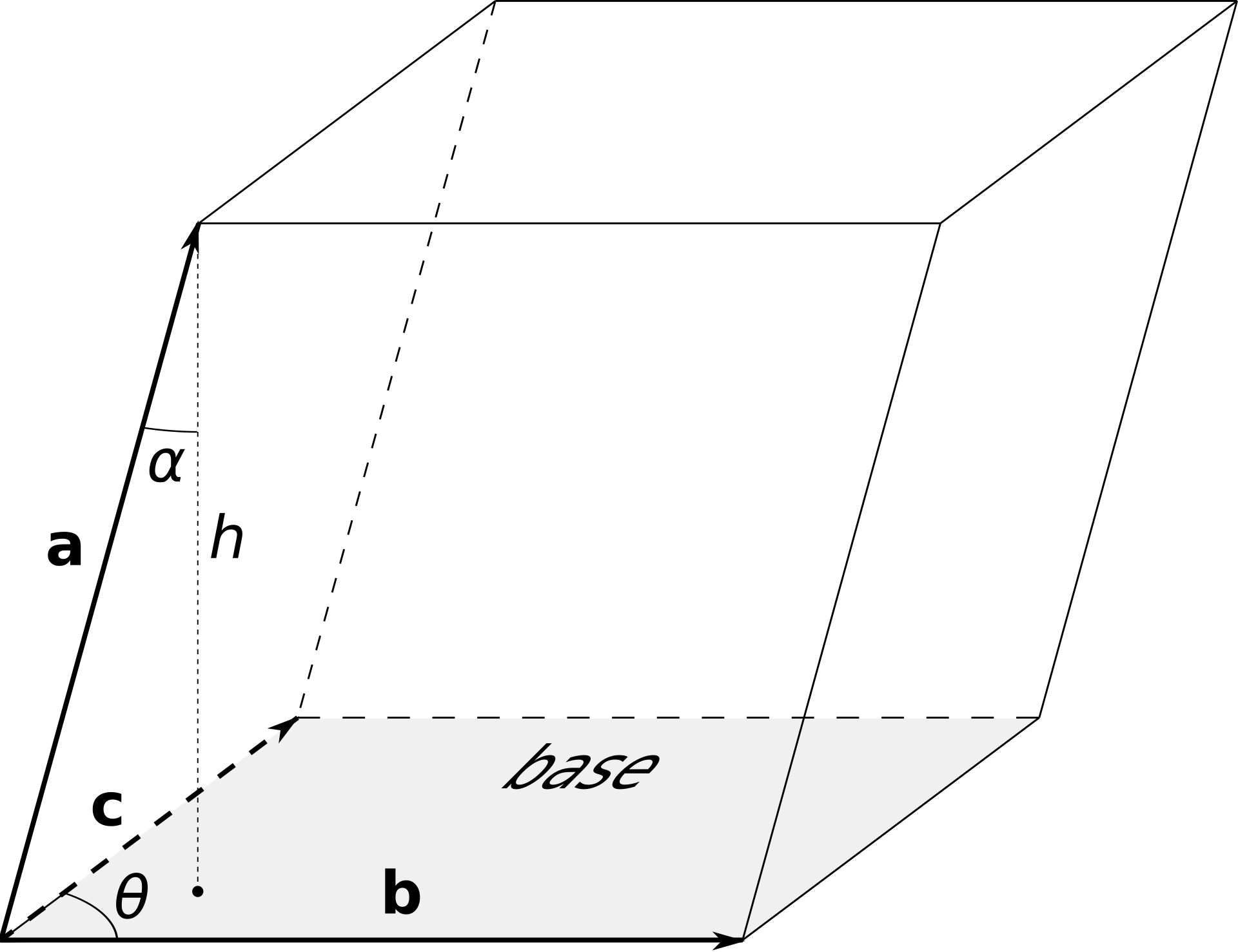
Vector triple product
Triple products are combinations of cross and dot products.
-
Scalar triple products: the magnitude of this is the volume of the parallelepiped (3D parallelogram) generated by , and .
-
Vector triple products: there's no easy geometric interpretation of this, but is useful to reduce complex cross product calculations. It can be memorized by the mnemonic BAC-CAB.
Spatial vectors
The position vector indicates the position of a point relative to the origin.
 In electrodynamics, usually we'll have two points: one for the source charge and one for the test charge. The vector from one to the other is the useful quantity then.

The Del Operator
Del () is a vector operator that acts upon functions, and is defined as really only is meaningful when applied to functions, and has three (usual) ways of being applied:
- To a scalar function () to get the gradient of that function.
- To a vector function via the dot product () to get that function's divergence.
- To a vector function via the cross product () to get that function's curl.
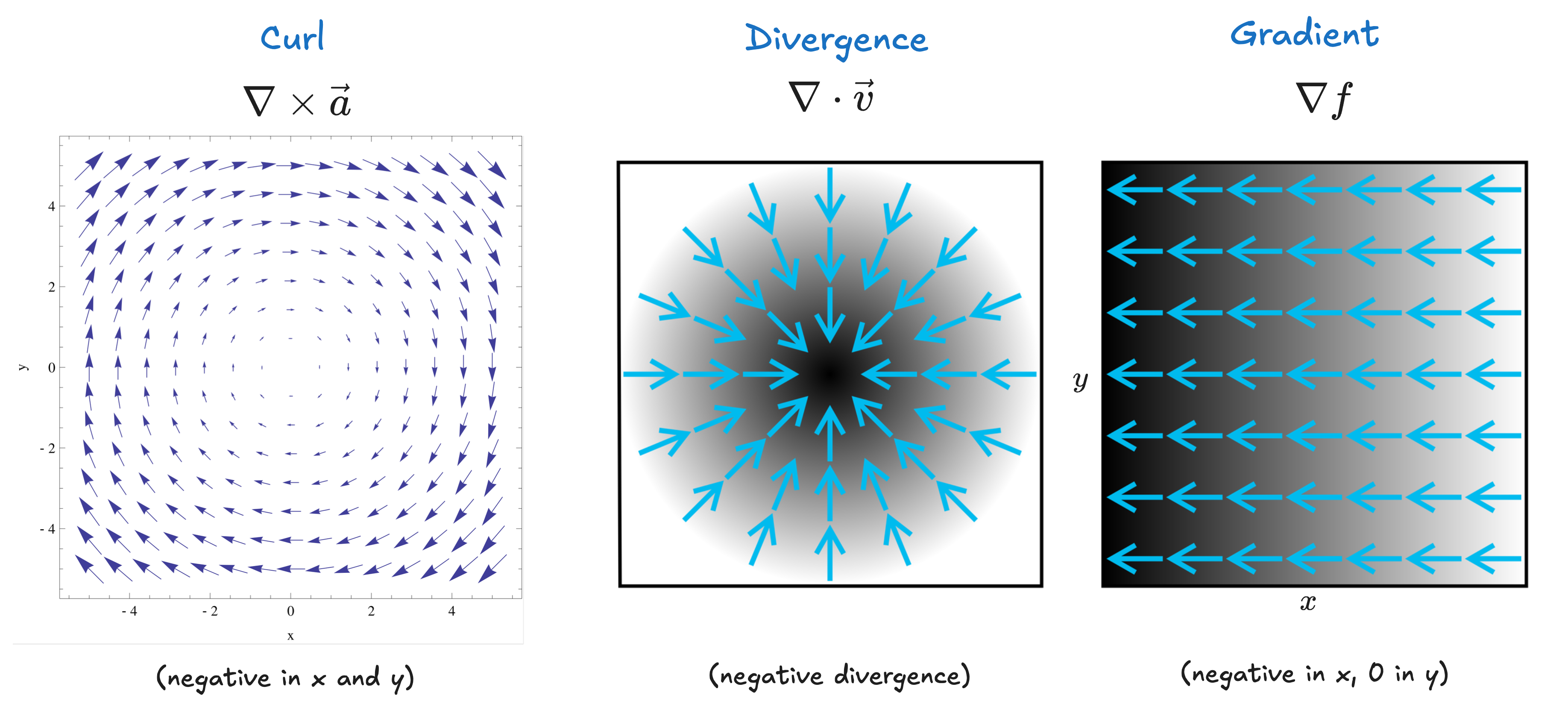
Gradients
The gradient of some scalar function gives a vector result that will point in the direction of the max rate of increase of that function.
and results in a vector with the derivative of the original function's units.
Fundamental theorem for gradients
Important: The integral of a derivative (here, the gradient) is given by the value of the function at the boundaries and .
Divergence
The divergence of some vector function represents how much the function "spreads out" or diverges from a given point. and results in a dimensionless scalar value indicating the rate of divergence from a point.
Green's theorem
Green's theorem is a special application of Stoke's theorem (see below). Geometrically, it relates the sources contained in some surface to the flux emitted by those sources around the boundary of a surface. In the case of electrostatics, this might be the flux field generated by some charges in a volume to the total, superposition flux coming out of that entire region - turning one "field of charges" into a single charge.
The integral of a derivative over some region will always be equal to the value of the function at the boundary () - in this case, the boundary term is an integral (a simple line may just have two endpoints, but a line bounding a volume forms a closed sufrface).
Curl
The curl of some vector function represents how much the function "swirls around" some given point. Positive curl is given by the right-hand rule (normally counterclockwise).
Stokes' Theorem
The integral of the curl over some surface is the "total amount of swirl" on that surface - and mathematically can be distilled into just finding how much the flow is following the boundary of that surface. This last quantity, is sometimes called the "circulation" of some vector field .
A Note on Del Squared ()
Enumerating over the ways we can apply twice:
- Laplacian: the cross product of with the gradient of a function results in the Laplacian, such that
- Curl of gradient: always zero.
- Gradient of divergence: not a lot of physical applications, calculable though.
- Divergence of curl: always zero.
- Curl of curl: most easily defined as the acceleration of the swirl, like a hurricane speeding up.
Integrals
In electrodynamics, we have line (path) integrals, surface integrals (or flux) and volume integrals.
Line integrals
Iterate over infinitesimally small displacement vectors . If , the line integral iterates over a closed loop and we can write
In elementary physics, a common example is work done by a force.
While path taken normally matters (distance), there are some vectors where only displacement matters (for forces, these are called conservative forces, like gravity).
Wikipedia has a really cool animation of line integrals:
Surface integrals
Surface integrals iterate over infinitesimally small areas , with norms perpendicular to the surface.
In this case, if the surface is closed (i.e. like a sphere, rather than a hill), then we can write it in closed loop form.

Surface integrals are really useful for things like flux where something is moving through some area - i.e. imagine radio waves passing through a curved gas cloud or radiation falling "through" a planet.
Volume integrals
Volume integrals integrate over infinitesimally small volumes .
If some function represented density of a substance, then the volume integral over it would be total mass.
Integration by Parts
Also known as the "inverse product rule".
Curvilinear Coordinates
Taking another look at spherical and cylindrical coordinates, as well as how to convert between them.
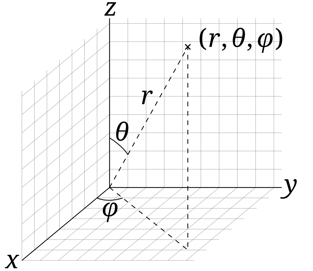
Spherical coordinates
Three terms:
- : the distance from the origin (range 0 to )
- : the polar angle from the -axis (range 0 to )
- : the azimuthal angle along the -axis (range 0 to )
Alternatively in terms of the unit vectors:
The interesting thing about the matrix form is that it is orthogonal - according to the invertible matrix theorem, for orthogonal matrices.
We can use this to solve for , and easily then by just taking the transpose of the above matrix.
Our line element in spherical coordinates is
In terms of triple integrals, the textbook has a good graphic to represent the three displacements .
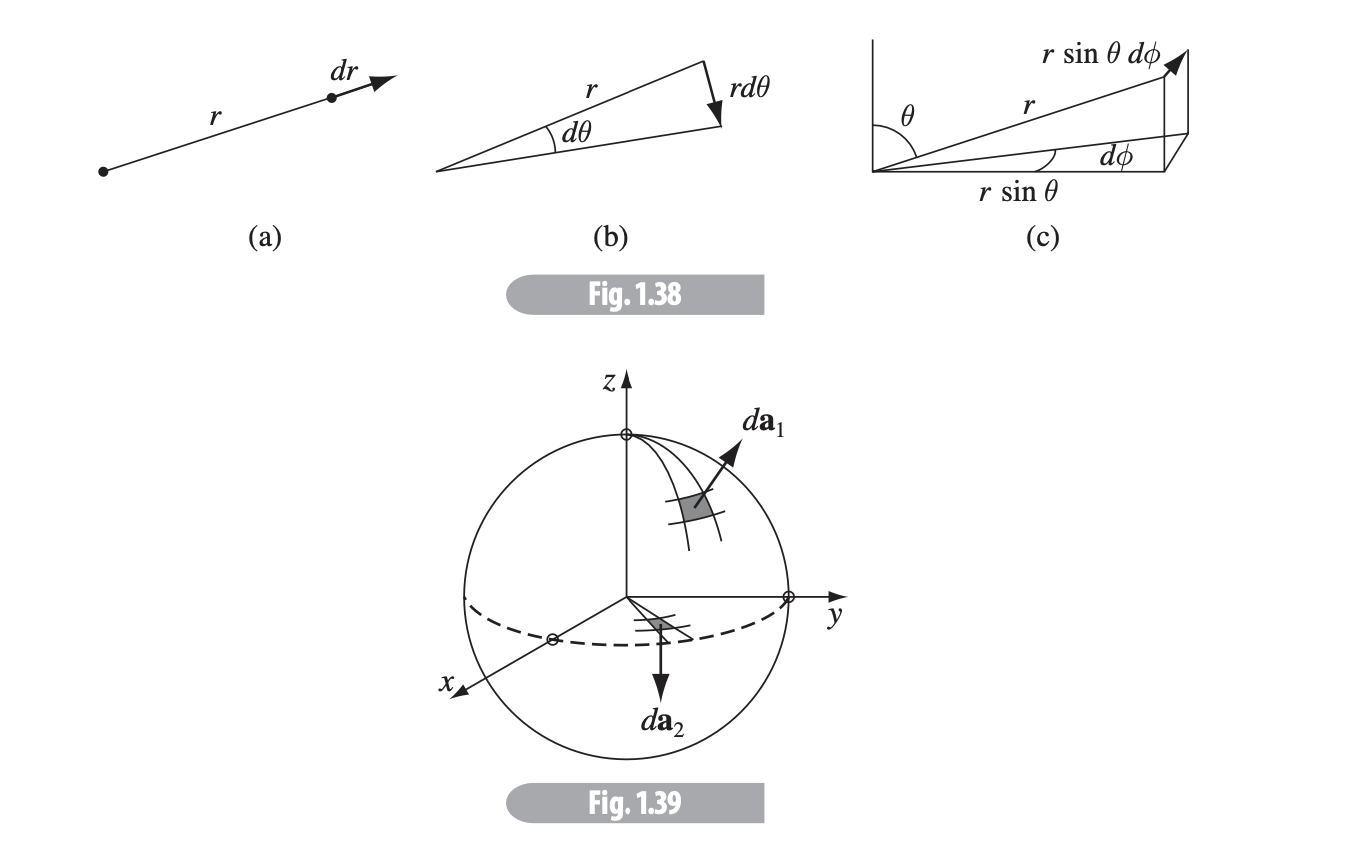
And a infinitesimal volume element is the product of these three:
has a possible range from 0 to , from 0 to and from 0 to .
The textbook represents the spherical representations of the gradient, divergence, curl and Laplacian in eqs. 1.70-1.73.
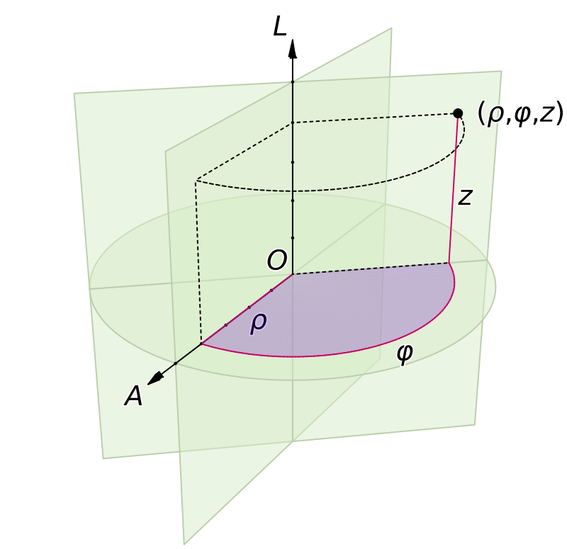
Cylindrical coordinates
Three terms:
- : distance from -axis
- : azimuthal angle along -axis
- : height along z-axis
 with unit vectors
For triple integrals, the infinitesimal displacements are our volume element is and line displacement is
Dirac Delta Function
Imagine we have an infinite point mass at the origin, and it is the only thing in the universe.
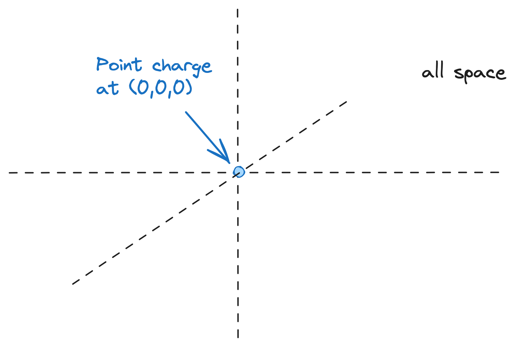 The total mass of the universe must be just the mass of the point charge; but the point charge exists only at , and is a point charge - it has no spatial dimension. If we were to integrate over the entire universe, we'd find we have just the mass of the point charge - and can mathematically represent that with the Dirac delta function.
and Therefore, if we have some continuous function (could be a constant or a function, anything attached to ). which brings us to the neat and nice identity:
Dirac Delta in 2D, 3D
And, unsurprisingly,
Note on : with (the separation vector), and Reference the textbook equations 1.100-1.102 for derivation.
Chapter 2 - Electrostatics
Reference "Introduction to Electrodynamics" by David Griffiths.
Fundamentally, electrodynamics seeks to model the interaction of some set of charges on some other charge, .
 We can do this via superposition, which states the interaction between two charges is unaffected by the presence of others - i.e. , the force between and , is independent of the presence of and . We can then sum up the forces to get our net force on :
In an electrostatic system (no moving charges as opposed to an electrodynamic system), the forces can be calculated via Coulomb's law.
We can do this via superposition, which states the interaction between two charges is unaffected by the presence of others - i.e. , the force between and , is independent of the presence of and . We can then sum up the forces to get our net force on :
In an electrostatic system (no moving charges as opposed to an electrodynamic system), the forces can be calculated via Coulomb's law.
Coulomb's Law
Electrostatics simply takes into account distance and charge strength. Coulomb's law is
is the permittivity of free space ( and (Griffith's script-r).
in electrostatics, force increases with higher-magnitude charges, and decreases with distance.
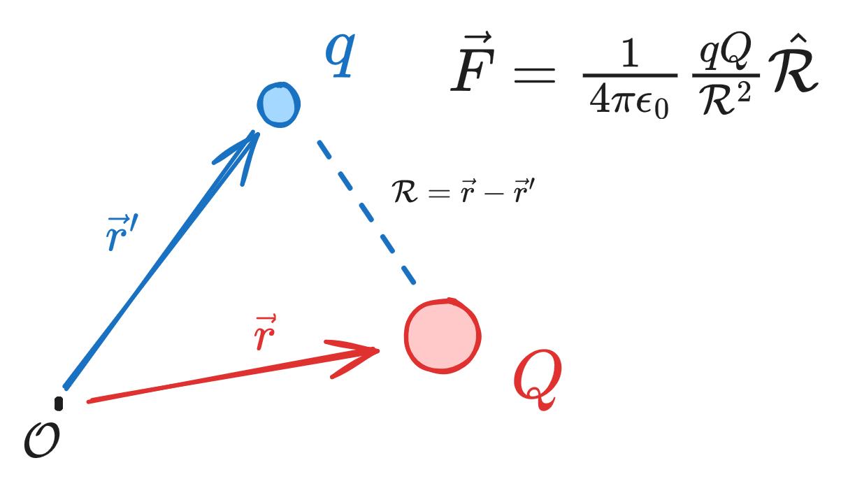 If we have several charges, we just sum their individual Coulomb forces as calculated above:
In shorthand, where , the electric field, is where .
The electric field is the force per unit charge - this force can only be imparted by the presence of other charges.
Continuous Charge Distributions
If we have a set of charges , then our electric field is generated from a discrete charge distribution. If, however, the charge is distributed continuously over some region, then we have a continuous charge distribution generating the -field.
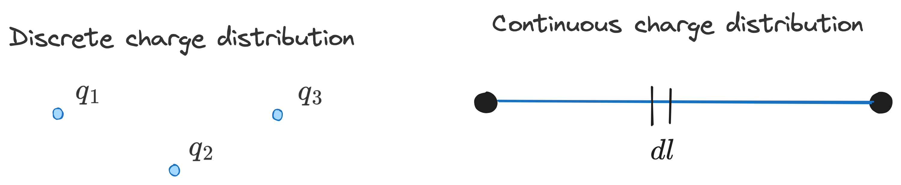 The electric field calculated as an integral over that continuous distribution:
where varies for our continuous distribution type (1D, 2D or 3D), such that:
The electric field calculated as an integral over that continuous distribution:
where varies for our continuous distribution type (1D, 2D or 3D), such that:
- Line:
- Area:
- Volume:
Regarding the vectors,
- is from the origin to test point; above a disk, this might be be .
- is from the origin to infinitesimal elements; often or .
- , .
The will usually yield two unit vectors (i.e. ). Use two separate integrals with the same element to handle.
Divergence and Curl of Electrostatic Fields
Griffiths 2.2.
Field lines are a way to visualize electric fields on a 2D or 3D medium.
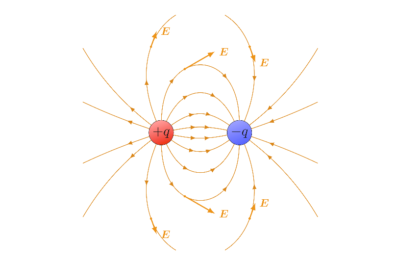
where the density of field lines indicates the strength of the E-field at that location (strongest near the center in the above image). The flux of through some surface is and is a way to measure the total charge contained within a closed surface, while those outside of the surface don't affect it.
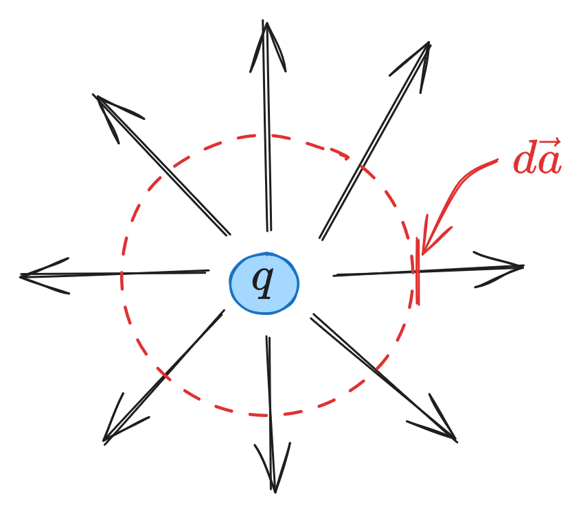
This mathematically represented by Gauss's law, which states There's also a differential version of Gauss's law (found by applying the Divergence Theorem) where is charge density:
For example: in 3D, if a point charge is at the origin then the flux of through a sphere around it is
We're only evaluating at the surface of the sphere, so is constant.
Note that Gauss's law is only useful with objects where the E-field is pointing in the same direction as elements . This requires both a symmetrical charge distribution within the object, and for the Gaussian surface to be symmetric according to one of the following:
- Spherically symmetric (concentric spheres)
- Cylindrically symmetric (coaxial cylinders)
- Plane symmetric (like a "box" that is cut in half by the plane)
The associated coordinate system is used for each.
Note: flux from external charges is ignored, since the flux entering a Gaussian surface from an external charge will be equal to the flux leaving that surface from the other side - hence, net flux from those external charges is zero.
If the object we're evaluating doesn't have perpendicular surface elements (i.e. a charge at the north pole of a sphere instead of the center), then some problems can be approached by creating another Gaussian element centered over the charge which subtends the same angle, though this can get geometrically complicated.
Divergence of
Since , then this just becomes Or, in shortform,
Curl of
For any electrostatic charge distribution, the curl of the field is always zero.
Electric Potential
Griffiths 2.3.
Electric potential is a good indicator of the "strength" of an electric field between two points, and is defined as with units .
A "natural" origin is a point infinitely far from the charge, though only when the charge distribution itself doesn't also extend to infinity.
in differential form, it's the reverse: Voltage is path-independent and only displacements matter - hence the electric potential between points and is
Poisson & Laplace Equations
Poisson's equation says If there is no charge (), Poisson's equation turns into Laplace's equation:
Voltage equations
For a point charge
is the reference point from origin, from the reference point to the infinitesimal charge (or reference point to point charge).
For a set of point charges, we can use the principle of superposition:
For a continuous distribution, and for a volume (to compute when we know ):
Note: this is similar to the formula for electric field, but is missing . is a scalar quantity, directionless.
Note on continuity
For some surface,
- The normal component of is discontinuous by some amount at a boundary.
- So, if the surface is uncharged (), is continuous across the boundary.
- The parallel component of is continuous (). Representing both, The electric potential is always continuous across any boundary (however the gradient of inherits the discontinuity in , since ).
Summary
The three "fundamentals" of electrostatics are , and , and are related by the following:
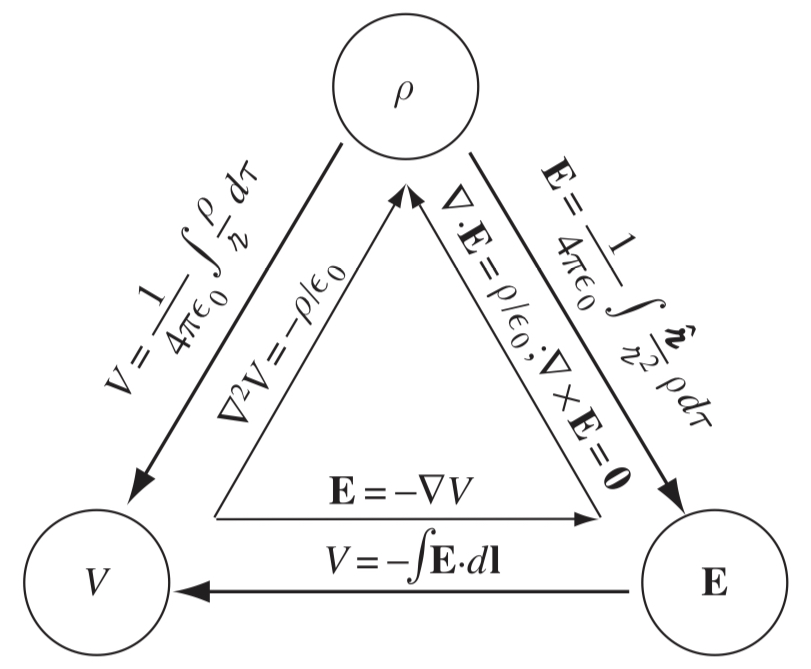
Griffith's Fig. 2.35.
Work and Energy
Griffith's 2.4.
For a conservative force, work is force times displacement. In electrostatics, our equivalent version is
More extended,
where work here is the work it takes, per unit charge, to carry a charge from to . If our reference point and we let , then
Work in a Point Charge Distribution
Imagine we had some charge - then brought in a new charge to join . Our work done would be
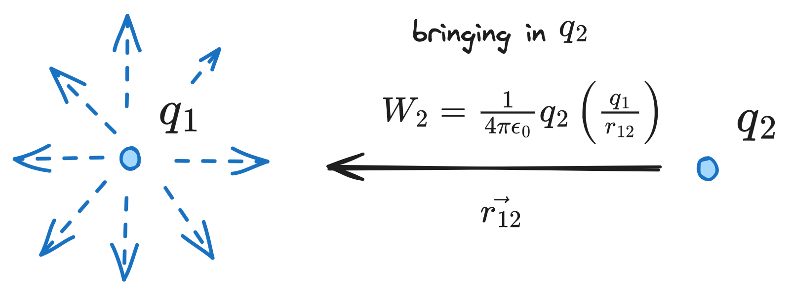
It would cost Then, to bring in a third charge would act against the superposition of and : ... etc. To assemble charges, we'd need a work of
Work in a Continuous Charge Distribution
For a continuous charge distribution, we use our last equation for our point charge distribution system and replace the sum with an integral .
Note: is not volume, but potential. This can be done via Gauss's law as well, see this hyperphysics article.
With a bit of mathematics, this is equivalent to
Conductors
Griffith's 2.5.
Conductors are materials in which electrons are free to roam (like cows, on an open ranch 👍). In contrast, insulators have electrons pretty much immobile and packed-together (like Monsanto farms 👎).

We can approximate metals as ideal-case conductors (though perfect conductors don't yet exist, though we're gradually coming closer) with the following attributes:
- inside a conductor - or, the induced field will cancel the external field. If an external field is applied to a conductor, free electrons will move toward the E-field until they all sit on the surface, creating a deficit of charges on the opposite surface and positively charging it.
 Crucially, the net E-field is zero, so the fields must cancel inside:
Charge will continue to flow until the cancellation is complete. Outside the conductor, , since the two fields don't tend to cancel.
Crucially, the net E-field is zero, so the fields must cancel inside:
Charge will continue to flow until the cancellation is complete. Outside the conductor, , since the two fields don't tend to cancel. - Charge density is zero : Since Gauss's law says , zero E-field means zero charge density in the conductor.
- Net charge resides on surface: positive and negative charges will only sit on the surface after enough time passes.
- is perpendicular to the surface: somewhat obvious, but bears mentioning.
Any dynamical system will try to minimize potential energy - the charges residing on the surface are an extension of this. It might take some time, but will eventually happen.
Induced Charges
If we hold a charge near a conductor, the conductor will move toward the charge - this is because negative charges will accumulate closer to than the "effective" charges on the far side. Force falls off by , so the conductor will be attracted to the charge.

Cavities
Let's say we have a cavity inside our conductive surface. There are two scenarios here:

Empty cavity: If the cavity has no charge, the field within the cavity is zero, regardless of the external fields applied. This is the principle of the Faraday cage.
Non-empty cavity: The charge contained by the cavity will induce an opposite charge uniformly distributed on the walls of the cavity - the only information transmitted to an external observer is the distribution of charge on the exterior wall (i.e. the magnitude of the internal E-field, or the amount of net charge contained).
Surface Charge and Force on a Conductor
Through the field inside a conductor is zero, the field immediately outside is
If we only care about the magnitude of the E-field, then .
However, the electric field is discontinuous at a surface charge, so when calculating the force per unit area (or pressure) of an E-field at the surface of a conductor, we average the E-fields above and below the surface, such that This is the outward electrostatic pressure on the surface, tending to draw the conductor into a given field, regardless of the sign of (squared away).
The pressure at this point, expressed in terms of the field just outside the surface, is
Capacitors
Put two conductors beside one another, with equal and opposite uniform net charges on one and on the other:
 Since the charge density is uniform on each surface, (on the left plate) and the field between the two is
with a voltage of
Since the charge density is uniform on each surface, (on the left plate) and the field between the two is
with a voltage of
in a uniform E-field.
We'll define a new term to represent the proportionality of the arrangement, capacitance: with units of Farads , usually expressed in or . The work to go from one side to the other is
Chapter 3 - Potentials
Reference "Introduction to Electrodynamics" by David Griffiths.
The goal of electrostatics is to find the electric field given some stationary, immobile charge distribution.
Coulomb's Law is the way we do this for simple charge configurations, but for more complex charge configurations it's often easier to work with potential . For areas of nonzero charge density such as point, surface or volume charges, we use Poisson's equation: Outside of these charge regons (such as in regular space), this reduces to Laplace's equation: with solutions called harmonic functions.
Laplace's equation is fundamental to the study of electrostatics according to Griffiths.
Laplace's Equation
 In three dimensions, visualization is challenging - but the same two properties apply, with the first this time being
- The value of is the average over a spherical surface of radius centered at that point, with
- can have no local maxima or minima, with extreme values only permitted at the boundaries (i.e. surface of the sphere).
Point 2 is particularly relevant in each of these circumstances - the value of at some point is the average of the surrounding on some surrounding boundary.
Uniqueness Theorems
The proof that a proposed set of boundary conditions will suffice takes the form of a uniqueness theorem (alternatively, a criterion to determine whether a solution to the Laplace or Poisson equations is unique).
Uniqueness Theorem 1: the solution to Laplace's equation in a volume is unique if is specified on a boundary surface enclosing the volume .

The surface does not have to be Gaussian - it can look totally eldritch and crazy and the theorem would hold.
Uniqueness Theorem 2: given a volume surrounded by conductors and containing some charge density , the electric field is uniquely determined if the total charge on each conductor is given.
Method of Images
Griffiths 3.2.
Say we have some charge a distance above an infinite grounded plane; what is the potential in the region above the plane? Our boundary conditions state
We could solve Poisson's equation for this region, but a much easier technique is to use the Method of Images. Wikipedia says on the subject:
The method of image charges is used in electrostatics to simply calculate or visualize the distribution of the electric field of a charge in the vicinity of a conducting surface.
It is based on the fact that the tangential component of the electrical field on the surface of a conductor is zero, and that an electric field E in some region is uniquely defined by its normal component over the surface that confines this region (the uniqueness theorem).
Start by removing the conductor, and placing an opposite charge at :
 Then, the potential is easy to calculate:
which obeys both of the boundary conditions of the original problem:
Then, the potential is easy to calculate:
which obeys both of the boundary conditions of the original problem:
- when
- for
Thus by uniqueness theorem 1, is the solution to our original problem.
Uniqueness theorem 1 means that if a solution satisfies Poisson's equation in the region of interest and assumes the correct value at the boundaries, it must be right.
The Method of Images can be used in any scenario where we have a stationary charge distribution near a grounded conducting plane.
Induced Surface Charges
The surface charge density induced on a conductor is where is the normal derivative of at the surface. In the above case, this is is in the direction - if we take this partial derivative of our above calculated voltage, then
As expected from a positive charge, the induced surface charge is negative and greatest at .
The total induced charge is Yes!
Force & Energy
Since the induced charge on the conductor is and our charge is , it is attracted to the plane with a force given by Coulomb's Law: While force is the same in our mirror problem, energy is not. For two point charges, , such that But for a single charge and conducting plane (continuous charge distribution), energy is half of this.
The work to bring two point charges towards one another does work on both of them, while to bring a point charge toward a grounded conductor has us only doing work on one charge - only half the work is necessary.
Separation of Variables
Griffiths' 3.3
Separation of variables is a way to solve ODEs and PDEs by rewriting equations such that each of the two variables occur on different sides of the equation.
Separable equations must be able to be written in the form We can rearrange the terms to get integrate, and add some constant term to one side to represent all our constants of integration.
In the context of electrostatics, separation of variables is very useful when solving 2D Laplace equations, such as We need solutions in the form of This can be accomplished through some mathematical trickery to find our separated variables ... ... which is of the form . Thus, both and must be constant (we can't hold one constant and change the other with this solution still holding).
So, Converting each equation into an ODE, ... we converted a PDE into two ODEs, which are much easier to solve. Our solutions will be a constant coefficient set: We can find our constants based on our boundary conditions now.
Multipole Expansion
Griffiths 3.4
Say you have some charge that you can see in space, far away. is almost like an exoplanet in a sense: we know it exists, we know its total mass, and maybe we know stuff like how far away it is.
But, we don't know what the surface looks like; what it's composed of, be it rock or ice or water. Just its net mass.
 Similarly, our charge distribution might be crazy complicated, and it's net charge only describes a tiny part of the story, albeit an important one - the multipole expansion is used to describe this fuller story, and is defined in terms of voltage as
Thus, the monopole moment is stronger than the dipole moment, the dipole stronger than the quadrupole moment, and so on.
Mathematically, it is where is the angle between and , is the reference point (from origin) and the charge (from origin).
Electric field of moments: the electric field is defined as .
To find the electric field i.e. caused by the dipole moment, find the voltage term for that dipole moment, then take the negative gradient of it.
Monopole and dipole terms
At large , a charge distribution just looks like a net charge (like an exoplanet). Thus, the monopole moment is just the net charge: The dipole moment describes the individual distribution of charges:
points from the origin to some charge distribution. is from the origin to some reference point.
Origin of coordinates
Changing the origin will never change the monopole moment , but will change the dipole moment as long as the total charge .
For example: if our system has and as its point distribution, and the dipole moment is origin-independent.
Chapter 4 - Electric Fields in Matter
Reference "Introduction to Electrodynamics" by David Griffiths.
This chapter looks at electric fields within matter that aren't necessarily conductors - i.e.most matter in the universe.
Polarization
Griffith's 4.1
If we place a neutral atom in an electric field, the net force on it is zero (as it is uncharged) - however, the positively-charged nucleus is pushed along into the field, while the negatively charged electron cloud is pulled down into the field.

The neutral atom is now polarized, with some tiny dipole moment : is the atomic polarizability and varies from atom to atom.
If the electric field is strong enough, the cloud will be ripped away from the nucleus and the atom will become ionized. Coulomb's law determines both.
Molecules become more complicated, since they're a few individual atoms coupled together - CO for instance has different polarizabilities parallel or orthogonal to its axis (), so for molecules, a polarization tensor might be more useful.
Force on dipoles
In the presence of an electric field, a dipole will rotate to point in the direction of the -field with a torque given by
At any other point on the dipole than the origin, .
 The net force on a dipole in a uniform field is zero as seen in the first image. However, in a nonuniform electric field, the force on a dipole is
The potential energy of a dipole in an electric field is
The net force on a dipole in a uniform field is zero as seen in the first image. However, in a nonuniform electric field, the force on a dipole is
The potential energy of a dipole in an electric field is
The Field of a Polarized Object
Griffiths 4.2
In the presence of an external electric field, the individual atoms of a given material will become polarized, leading to a lot of little baby dipoles, all pointing in the direction of the applied field.
Since all of its constituent atoms are polarized, the material itself is said to be polarized with some polarization density .
Potential
Since the potential for an individual dipole is The electric potential for the entire object with polarization is With surface and volume bound charge densities of We can rewrite the potential of our whole polarized object in terms of these densities:
The net potential is just the sum of the potentials produced by the bound surface and volume charges.
, where is the angle between and . in spherical.
To calculate the electric field caused by polarization, use
Physical interpretation of bound charge
Say we have a long string of dipoles, as we might in a polarized dielectric in some field . The head of one dipole will cancel the tail of its neighbor, except at the ends, so that:
 No one electron makes the whole trip - but the magnitude of the in some field will be matched by , such that it's almost conductor-like - in a uniform field, we see only accumulations of bound charge on the surface, such that
If, however, the polarization is non-uniform, then we'll see accumulations of bound charge within the object, as well as on the surface,
No one electron makes the whole trip - but the magnitude of the in some field will be matched by , such that it's almost conductor-like - in a uniform field, we see only accumulations of bound charge on the surface, such that
If, however, the polarization is non-uniform, then we'll see accumulations of bound charge within the object, as well as on the surface,
The Electric Displacement
Griffiths 4.3
Most materials aren't perfect conductors or perfect insulators. Conductors have free flowing electrons , while insulators have exclusively bound charges - a normal dielectric will have both free and bound charges, such that Let the displacement field take into account the fields of the polarization field and electric field, such that Gauss's law for is
We only have control over free charge - bound charge is a consequence of the properties of the material itself. Free charges themselves generate a field.
Though Gauss's law has a parallel for , Coulomb's law does not.
The curl of is
Boundary conditions
For a given dielectric, the boundary conditions are:
Note that since the curl of is zero ),
Linear dielectrics
Griffiths 4.4
For linear substances, the polarization is linearly proportional to the total electric field:
is the electric susceptibility of the medium (dimensionless), with being the permittivity of the material (with in vacuum, the permittivity of free space). A unit-less version is the dielectric constant, .
The displacement field in linear media is thus
Notes on examples
Example 4.5: conducting sphere of radius and charge surrounded by linear dielectric of radius and permittivity , find potential at the center.
- The conducting sphere of charge is our enclosed free charge, so
- Inside the sphere,
- Integral to find potential is (with reference to infinity):
Example 4.6: parallel plate capacitor filled with dielectric material of dielectric constant , what effect does this have on capacitance?
- Dielectric will reduce , and hence , by factor of
- Since , capacitance increased by :
Boundaries of linear dielectrics
In a homogenous isotropic (uniform) linear dielectric, : The boundary conditions are (for ): In terms of :
The potential above and below the boundary is continuous.
Energy in dielectric systems
The work to fill (charge) a capacitor is If a capacitor is filled with dielectric, the capacitance increases by ; thus the work does as well. The total work done (derivation in Griffiths 4.4.3) to fill the capacitor from 0 to its final configuration is
Work is still "energy to assemble a system".
Forces on dielectrics
Dielectrics are attracted into fields just as conductors are, since bound charge tends to accumulate near the free charge of opposite sign.
In a capacitor with a partially-inserted dielectric, this might look like this:
 Fringing fields are "notoriously difficult to calculate" (agreed!) - see Griffiths 4.4.4 for a method to deal with them, the result of which is
where is the width of the plates (for a square plate, ).
Fringing fields are "notoriously difficult to calculate" (agreed!) - see Griffiths 4.4.4 for a method to deal with them, the result of which is
where is the width of the plates (for a square plate, ).
Useful Equations
Here are (most) of the equations I found useful in this class.
Dimensional analysis
Symbols: time (T), length (L), mass (M), electric current (I), charge (Q = TI), energy (TLM)
| Thing | Dimensional units |
|---|---|
Wikipedia's dimensional analysis page has some other good simple cases.
Electrostatics
Coulomb's law (both and )
Notes:
- points from the origin to point we're interested in, from the origin to some 'unit charge' , thus .
- Imagine from one point charge to another.
Gauss's law
Multipole expansion
Monopole moment is total charge Dipole moment points from south to north, origin-dependent Quadrupole moment describes how charge dist. behaves in nonuniform fields
, the charge integration element, is
The electric potential for all multipole expansion terms is
- represents the th Legendre polynomial
- is the angle between and
Legendre polynomials
Calculated according to Rodrigues' formula:
| 0 | |
| 1 | |
| 2 | |
| 3 | |
| 4 | |
| 5 |
Del operator
Due to unit vector and coordinate conversions, has different representations as applied in divergences as compared to normal functions.
| Coordinate system | Gradient of | Dot product with |
|---|---|---|
| Cartesian | ||
| Cylindrical | ||
| Spherical |
Chapter 5 - Magnetostatics
Reference "Introduction to Electrodynamics" (5e) by David Griffiths.
Say instead of static electric charges (electrostatics), we start dealing with moving electric charges (electrodynamics).
Moving charges will generate a magnetic field around them. If the rate of moving charges (current ) is constant, we're working with magnetostatics. The -field for some current can be modeled by the right-hand rule:

Magnetic fields interact with one another. Using the Lorentz force law, Or, in the presence of an electric field as well,

Magnetic forces themselves do no work: This means that magnetic forces can change the direction of a charged particle in motion but cannot speed up or slow them down.
Cyclotron motion
Cyclotrons are varieties of modern particle accelerators - cyclotron motion is the motion a charged particle has moving around some central axis:
 and adheres to the cyclotron formula:
with some cyclotron frequency given by
and adheres to the cyclotron formula:
with some cyclotron frequency given by
If the particle has some velocity component parallel to the -axis, , the circle will look more like a helix (see this visualization), since there is no parallel component along the axis of the Lorentz force law (for this scenario).
Current
Current is some charge per unit time through some cross-sectional area, defined such that If we had some line charge of Coulombs traveling at velocity , . In cases where we're not just along a straight line, is a vector and as such current is too: The force on this line of charge is for a constant current .
Surface and Volume Currents
If we have some charges flowing across some on a surface, or across some area on a volume, we represent them with surface current density and volume current density .

and are both perpendicular to the direction of current flow.
Similar to a line charge, if our surface has density (or for a volume charge) and charges move at velocity : For some volume, the charge conservation equation (or continuity equation) says any charge flowing out of a volume means
Note: means change in charge density per change in time, meaning . This is zero in magnetostatics.
Biot-Savart Law
The magnetic field of some steady-state line current is
Note: has units of newtons per ampere-meter (or Tesla): .
where is the "test point" where you'd like to know the magnetic field, points to some (temporary) infinitesimal charge line element , and points from the charge element to the test point.
 Note: the integration is along the current path.
is the "permeability of free space":
The B.S. law also works for surface and volume charges: where and , converting to polar or spherical as necessary.
Divergence and Curl of
The curl of any magnetic field is proportional to the current density (or contained current): where is a volume current density. It's also related to total current by taking a surface integral bounding the volume:
This means stronger currents have higher-magnitude -fields, and stronger -fields enclose a higher current / current density within.
The divergence of a magnetic field is always zero.
A magnetic field will circle around a wire but will not expand outward.
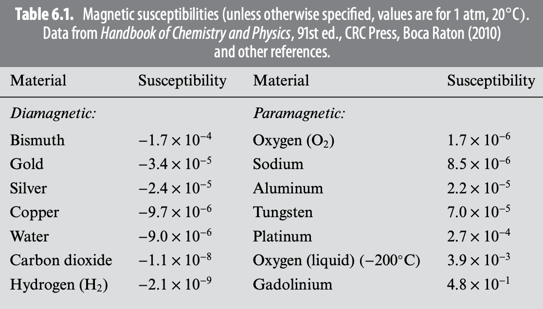
Ampère's Law
For some circular magnetic field (circumference ) around a wire, the path integral of it is independent of radius:
The radius of the path integral (circle, circ. ) increases at the same rate as the magnitude of the -field decreases - i.e. it's independent of radius.
This is known as Ampère's Law: The current enclosed by some path integral along the -field is proportional to the enclosed current . It's like the magnetostatics equivalent to Gauss's law as it relates to Coulomb's law.
 For a surface current along an infinite plane, the Ampèrean loop might be a rectangle perpendicular to the current.

Above, the components of the Amp. loop aren't aligned with , so we only care about the components - i.e.
Note that Ampère's law only works for
- Infinite straight lines / cylinders
- Infinite planes
- Infinite solenoids
- Toroids (see Griffiths Ex. 5.10)
For surface current densities (with perpendicular to ) and volume current densities (with similarly, see above).
Magnetic Vector Potential
Magnetic vector potential is the magnetostatics equivalent to electric potential .
. If we instead write this as , Griffiths has a further derivation of this in 5.4.1. Ultimately, we get to the magnetic Poisson's equation equivalent: We can pull out if constant. Use or for surface and volume currents respectively.
The direction of will almost always be the same as that of current.
Dipole Moment of
The explicit multipole expansion of is in Griffiths 5.4.3. I've only included the dipole moment for brevity, and because the monopole moment has no proof of existence & higher-order terms are rarely helpful.
The dipole moment tends to dominate magnetic vector potential multipole expansions (no monopole given ), and is represented as where is the magnetic dipole moment this is independent of origin, since is centered at .
Chapter 6 - Magnetic Fields in Matter
Reference "Introduction to Electrodynamics" (5e) by David Griffiths.
If a material is placed in a -field, it will acquire a magnetic polarization (or magnetization). Different materials acquire different polarizations depending on their atomic structures.
- Paramagnets: magnetization parallel to applied , materials with odd # of electrons.
- Diamagnets: magnetization antiparallel to applied , materials with an even # of electrons.
- Ferromagnets: magnetization persists on the material even after the applied -field is removed, and is determined by the whole "magnetic history" of the object.
All electrons act as magnetic dipoles.
Imagine a magnetic dipole as pointing from south to north (the Gilbert model). It's an inaccurate model at small scales according to Griffiths, but he recommends it for intuition.
Torques and Forces on Magnetic Dipoles
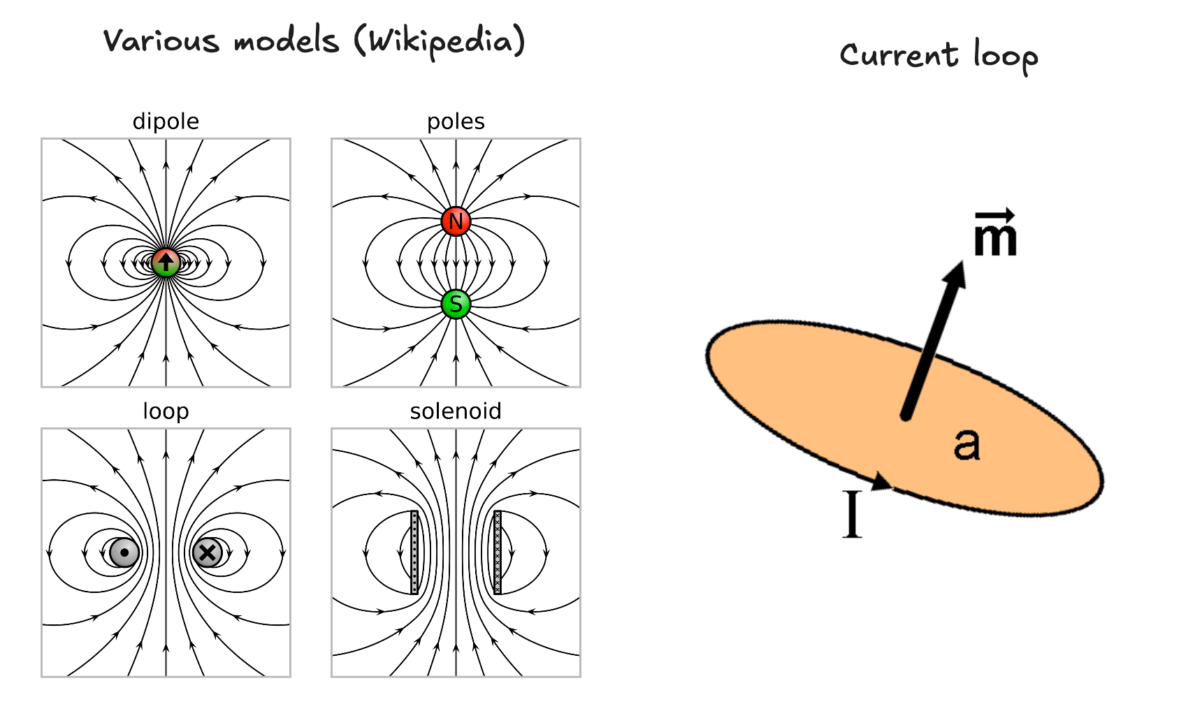
Magnetic dipoles will experience some torque in an applied field, where and is the magnetic dipole moment, defined (for current loops) as where is the "vector area" of the loop, which is just the enclosed area if the loop is flat. The direction of follows the right-hand rule.

In a uniform field the net force on the dipole is zero, though this is not the case for nonuniform fields.
For an infinitesimal loop with dipole moment in field , the force on the loop is
Diamagnets
Diamagnetism affects all materials, but is much weaker than paramagnetism, so is most easily observed in materials with an even number of electrons.
When an external -field is applied to a material, individual electrons will speed up according to where is the "radius" of the electron from the nucleus of an atom. This increase in orbital speed will change the dipole moment this change in the dipole moment is antiparallel to as shown above.
Magnetization
Magnetization is For a paramagnet, perhaps suspended above a solenoid, the magnetization would be positive/upward, and force downward. For a diamagnet, the magnetization would be instead downward, and force upward.
In general in a nonuniform field, paramagnets are attracted into the field, and diamagnets are repelled away.
Note: is an average over a wildly complex set of infinitesimal dipoles and "smooths out" the dipole into a macroscopic view.
Note: both diamagnetism and paramagnetism are quite weak compared to, for instance, ferromagnetism, and so are often neglected in experimental calculations.
Field of a Magnetized Object
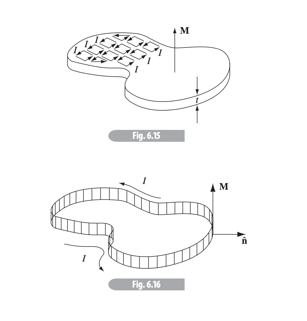
For some single dipole, the magnetic vector potential is For a magnetized object with magnetization , Alternatively, we can look at the object in terms of its volume current density and surface current density , where
This means the potential (and therefore magnetic field) is the same as would be made by some volume current throughout the material plus the surface current on the boundary.
This means we needn't integrate all the infinitesimal dipoles, but rather just determine the bound currents and and find the field they produce.
Note:
Auxiliary Field
The auxiliary field is, in a sense, the magnetic field since, it represents the real-world field we'd observe - including both the magnetic flux field and magnetism .
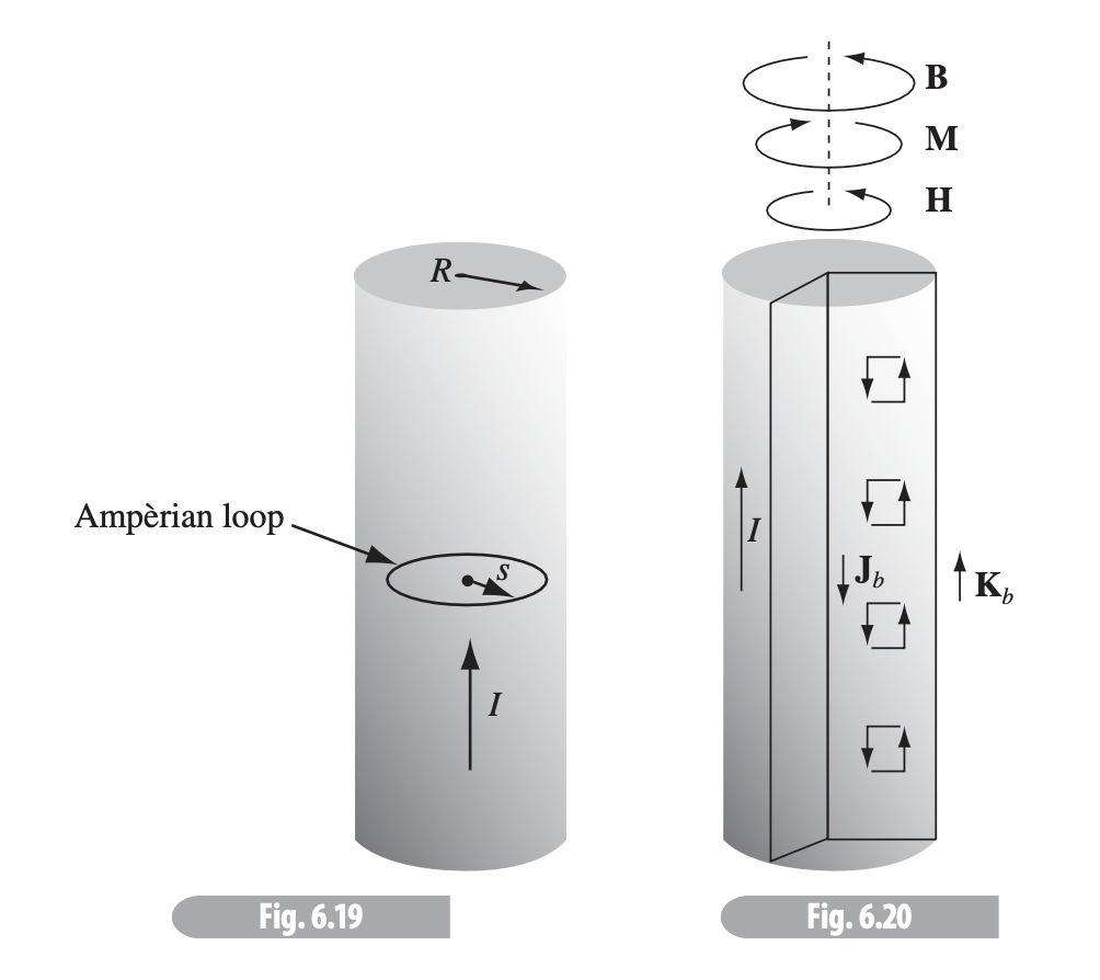
The free current is the current composed of moving free electrons (often caused by a battery or other current).
The bound current results from the magnetic polarization (magnetization) of individual electrons into dipoles - Griffiths represents each dipole as tiny current loops. Individually, the current loop of each individual atom tend to cancel one another out, except at the boundary where there are no adjacent atoms - thus the bound current density represents a current around the boundary of the surface (see this image).
"It is a peculiar kind of current, in the sense that no single charge makes the whole trip - on the contrary, each charge moves only in a tiny loop within a single atom. Nevertheless, the net effect is a macroscopic current flowing over the surface of the magnetized object." - Griffiths
The total current density is then the free-charge-current density plus the magnetized current density (or bound current). Ampère's law can be then written as
We can simplify by moving both curls to the left
This curl grouping is called the auxiliary field .
 Ampère's law becomes
where is the free current passing through the Ampèrian loop.
Ampère's law becomes
where is the free current passing through the Ampèrian loop.
We see when looking at a magnetometer. is difficult to isolate unless we know both the exact amount of current and/or the magnetic properties of the material, such that we can evaluate .
Note / warning:
, though more physically relevant in some ways, is harder to calculate:
- It has a non-zero divergence
- It cannot be calculated without knowing the material type
Symmetries
If you know the material type, this can be more helpful than the corresponding boundary conditions
Linear & Nonlinear Media
Linear media are those for which is linearly proportional to the magnetic field, .
This is the case for most materials, which tend to be either paramagnetic (odd # of electrons) or diamagnetic (even # of electrons), and the proportionality is (chi) is the magnetic susceptibility of a substance, and is:
- Positive for paramagnets.
- Negative for diamagnets.
- Dimensionless.
- Typically around .
Therefore Thus, , and where is the permeability of a material.
(the permeability of free space) is the case when .
is dimensionless.
To calculate in terms of and :
Ferromagnetism (nonlinear)
Ferromagnets require no external fields to sustain the magnetization, with each magnetic dipole pointing in the same direction as its neighbors.
However - this "pointing" only occurs in small patches called domains, with each domain cancelling the others out (usually), so not all iron devices are fully magnetic.

However, each domain will expand when placed in a sufficiently powerful magnetic field.
From Wikipedia: "Moving domain walls in a grain of silicon steel caused by an increasing external magnetic field in the 'downward' direction, observed in a Kerr microscope. White areas are domains with magnetization directed up, dark areas are domains with magnetization directed down."
If the field is strong enough such that one domain dominates, the iron becomes saturated. However, too-large domains are inherently unstable and will collapse into smaller fields without the presence of a large field, though the similar polarity will be present in each domain, so the iron remains magnetized until other fields affect it to go back to individual domains.
Ferromagnet design
Wrap a coil of wire around the iron to be magnetized, then run a current through it to generate a field. As increases, the domain boundaries move until they reach the saturation point.
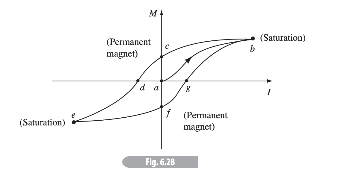 If we turn off the current, the permanent magnet remains. If we, however, run through the coil, we reverse the effect, as shown above, known as a hysteresis loop.
Ferromagnetic "history" may also be reset by increasing the temperature of the iron to 770 C, the Curie point - above this, iron also behaves more like a paramagnet.
Chapter 7 - Electrodynamics
Reference "Introduction to Electrodynamics" (5e) by David Griffiths.
Electrostatics is the study of the electric field of static electric charges; magnetostatics is the study of the magnetic field of moving electric charges. Electrodynamics is therefore the study of the electric field of moving electric charges.
Ohm's Law
To make a current flow, some force on the charges is needed - thus, current density can be written as proportional to the force per unit charge . Usually, the charge velocity is small enough that , so
This is a more primitive variety of Ohm's law, . Note that .
is the conductivity of a material, with the resistivity being
- Metals can be regarded as perfect conductors:
- Insulators/dielectrics:
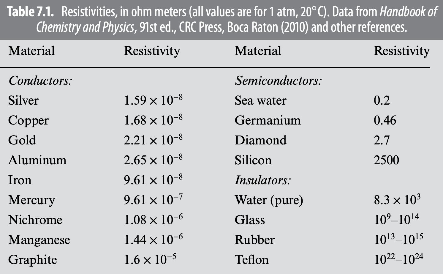
Resistors are made of low-conducting (hence high-resistivity) materials.
Actual resistance will depend on the dimensions of the material in question:
- is a quality of the material itself, while depends on the amount of that material used.
Power
Also known as the Joule heating law, power is measured in joules per second and is the amount of "energy" consumed by something, and is defined as
Electromotive Force
Now, regarding the EMF. Electromotive force (or electromotance) is not a force. Rather, it is the integral over the force per unit charge, or the forces driving each electron in a material, and is defined as , where is the 'source' or 'driving' force on each charge, usually a battery or something to create some potential difference , while "smooths out" the conductor such that we have an equal distribution of electrons everywhere (no buildups).
For an electrostatic circuit, and as such An ideal EMF source (resistanceless battery) has , so and thus
for an ideal EMF source (ideal battery).
is effectively the "work done per unit charge".
Motional EMF
When we move a wire through a magnetic field, we get a motional EMF.
From the Lorentz force law of a single charge moving through a magnetic field, EMF is force per unit charge , so This is fine, but can get complicated to calculate (as evidenced by homework 6). A much simpler way to calculate of some loop is via Faraday's law, where Here, is the magnetic flux, so is the change in magnetic flux through a loop.
EMF only happens when a loop and magnetic field are moving with respect to one another - i.e. if a loop moves further away from a source of magnetic field, or we move our line of current away from our loop.
Flux is really just the amount of magnetic field passing through some loop.
Induction & Faraday's Law
Michael Faraday noted some key things about induction - mainly:
A changing magnetic field induces an electric field.
This is represented by Faraday's law: In differential form, Thus, whenever the magnetic flux through a loop changes (or magnetic field changes w.r.t. a loop), an emf of will appear in the loop.
This emf is often called Faraday's Law of Induction - Griffiths disagrees but Griffiths is Griffiths.
Lenz's Law
In Griffiths' words,
Nature abhors a change in flux.

According to the Wikipedia definition on the subject, "[the] magnetic field created by the induced current opposes changes in the initial magnetic field."
Fleming's right hand rule is a good mnemonic to remember this:
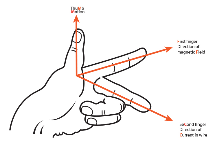
Induced Electric Field
Induced electric fields can be calculated in a manner similar to Ampere's law:
The rate of change of magnetic flux plays the same role as .
Mutual Inductance
Say we have two loops with the same current flowing through each.
 Let
Since both and are proportional to and respectively, we can rewrite this as
If as shown above, then
Let
Since both and are proportional to and respectively, we can rewrite this as
If as shown above, then
With the same currents, the magnetic flux through loop 2 () must be equal to the flux through loop 1 (), and
Since , with the same current and
Inductors

For several loops with constant current and mutual inductance , with
Energy in Inductors
If we start with and build it up to , the total work done is
Maxwell's Equations
Prior to Maxwell, we had four equations governing electric and magnetic fields:
However, these equations fail to account for two things:
- Ampère's law stops applying for nonsteady currents.
- , but (generally).
The key issue here is thus:
Changing electric fields induce magnetic fields, just as changing magnetic fields induces an electric field.
Maxwell added a "displacement current" term to "fix" Ampère's law: such that, now
This term is only visible in the presence of changing electric fields - magnetodynamics.
In terms of our "usual" form of Ampère's law,
The Equations
Chapter 8 - Conservation Laws
Reference "Introduction to Electrodynamics" (4e) by David Griffiths.
The mathematical equation for local conservation of charge (better known as the continuity equation) is
Poynting's Theorem
The total energy stored in electromagnetic fields is Poynting's theorem reads "the work done on charges by the electromagnetic force is equal to the decrease in energy remaining in the fields, minus the energy that flowed out through the surface".
It's easier represented by the Poynting vector: which represents the energy per unit time, per unit area or energy flux density.
represents the movement of energy or transfer of energy, and will point in the direction of this transfer.
The continuity equation for energy is
Momentum
Electromagnetic fields themselves carry momentum (bizarrely enough).
Imagine firing a gigantic laser beam from Earth at some spacecraft:
 The barrage of photon would cause the solar sail spacecraft to accelerate. This is the principle behind the Breakthrough starshot project. The only way this is possible is if the photons (i.e. the E/M waves themselves) carried some momentum.
Note on Newton's Third: in electrodynamics, Newton's third law (equal and opposite) does not always hold.
Maxwell stress tensor
The Maxwell stress tensor is used to relate electromagnetic forces and mechanical momentum, and is the force per unit area (or stress) acting on the surface.
The Kronecker delta is 1 if the indices are the same, zero otherwise, such that (for example):
The stress tensor can be written in two ways, both equivalent - the double arrow is used to indicate it's a vector with more than one index.
The dot product of the tensor can only operate under one index: The divergence of the stress tensor is ... long, but below.
The electromagnetic force per unit volume can be written and the total electromagnetic force on some charges in some volume is In the static case (i.e. does not vary with time),
In an applied context, is the force per unit area, in the th direction, acting on an element of surface in the th direction.
So,
- represent pressures.
- etc. represent shears.
Conservation of Momentum
Newton's second (in another form) says the force on an object is the rate of change in its momentum: The conservation of momentum in electrodynamics is therefore Griffiths' interpretation says the momentum stored in the E/M fields is while the second integral is the momentum per unit time, flowing into the volume through the surface.
The momentum density, or momentum per unit volume, is And the continuity equation for momentum is
Chapter 9 - Electromagnetic Waves
Reference "Introduction to Electrodynamics" (5e) by David Griffiths.
Griffiths defines a wave as "a disturbance of a continuous medium that propagates with a fixed shape at a constant velocity".
If we represent such a wave mathematically, then we can say that the displacement (from the origin) at some later time is Or just Solutions to this equation are determined via the wave equation. Let , such that . here the speed of propagation is given by Functions of the form are not the only solutions - the wave equation has the square of , so another class of solutions looks like - so the most general solution to the wave equation is
Note that this is a linear equation thus the sum of any solutions is also solution.
Waves that travel across some medium (like waves on an ocean or guitar string, moving with velocity ) are called transverse. Those that act more like a slinky are called longitudinal waves.
Sinusoidal waves
Sinusoidal waves take the form
- is the amplitude.
- is the phase constant.
- is the wave number, and is related to wavelength by
Cosine completes one cycle every .
The period is while the frequency (oscillations per unit ) Alternatively, the angular frequency can be more useful:
The direction of propagation is determined by the sign of . A leftward wave has , a rightward wave .
Complex wave notation
Waves can also be written in complex notation, by Or alternatively, with , The actual wavefunction is still given through the real component of this.
Polarization
Transverse waves move along a single axis (the direction of propagation):

Thus, there will always be two dimensions orthogonal to the direction of propagation given by the polarization vector , with the polarization angle . Most waves can therefore be considered a superposition of two waves: one horizontally polarized, one vertically, depending on your axis orientation.
Electromagnetic Waves
Derived from Maxwell's equations,
In a vacuum (outside of any material), replace and .
Both satisfy the wave equation in three dimensions: The velocity is given by
In vacuum, , the speed of light.
Monochromatic Plane Waves
"Monochromatic" implies the frequency is constant.
If these waves are traveling in a single direction and have no dependence on or , then they're called plane waves (fields uniform over every plane perpendicular to direction of propagation).
Useful Equations
Here are some of the equations and ideas I found useful in this class.
Magnetic Fields
from origin to test point, origin to test charge , (Griffiths' script-r)
| Scenario (current ) | Field | Griffiths ref. |
|---|---|---|
| Solenoid running along , turns per length | 5.59 | |
| Long straight wire of radius | 5.39 | |
| Center of a 4-sided square loop | pr. 5.8 | |
| Center of an -sided polygon | pr. 5.8 | |
| Center above a circular loop of radius | ex. 5.6 | |
| Center of a circular loop, | derived from above |
Magnetism
Force
For an electron .
Auxiliary field
is magnetic susceptibility, is permeability
:
Current densities and and surface density :
if uniform .
Divergence of curl is always zero.
Magnetic vector potential
Electrodynamics
Current density :
is current, current density, .
Electromotive force :
Dimensional analysis
Symbols: time (T), length (L), mass (M), electric current (I)
| Thing | Dimensional units |
|---|---|
| & | |
| () | |
| (conductivity) | |
| (vacuum permittivity) |
Del in other coordinates
In cylindrical,
In spherical,
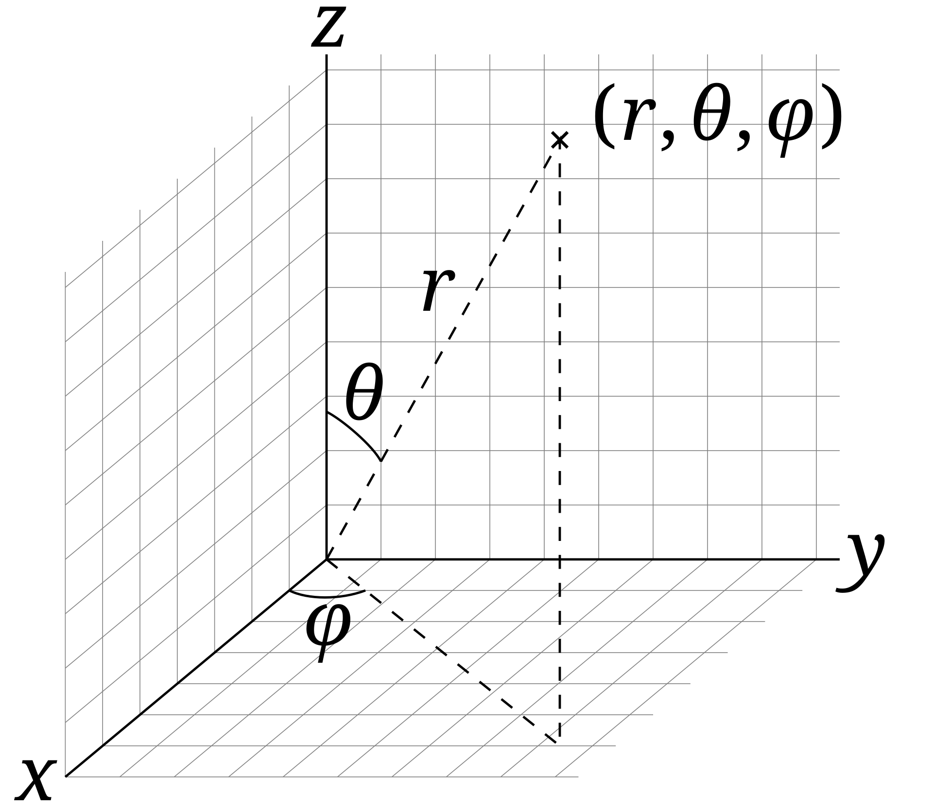
Mostly particles and symmetries. Probably ~2 questions on special relativity in the context of particle physics. 18 multiple choice, 2 long answer.
Special relativity
-
- is proper time
Group theory
indicate and commute together.
Transformation -> operator .
- If
- Continuous groups
- and
Rotation matrix in 3D
Spin
- e.g. is spin , up =
- is tensor product
- e.g.
Detectors
pc units of GeV, q units of , in , in
Prefixes!
| Unit | Equivalent |
|---|---|
| 1 GeV | 1000 MeV |
| 1 MeV | 1000 keV |
| 1 keV | 1000 eV |
| 1 eV | 1000 meV |
| 1 meV | 1000 eV |
| Minimum ionizing particle. Something? |
Geiger counters, phototubes, scintillators.
Particles
Lepton, neutrino, quark, Baryon, Hadron, meson
Symmetries:
Energy, momentum, Lepton (number, flavor), Baryon (number, flavor), charge
Forces:
- E&M (photons)
- Weak (W and Z bosons)
- Strong (gluons)
- Higgs (Higgs boso)
- Gravity (graviton?)
Decays and translations
"If it's weird enough to be weak then it's gotta be weak"
Ex.
Antineutrino?
Both strong and E&M decays conserve strangeness; how to differentiate?
- Any strong decay can also be E&M, but strong will be ... stronger.
- Cannot pick strong if involves leptons in photons
- If just a bunch of quarks, likely strong
- More complicated rules beyond this tho.
- Weak violates baryon flavor, doesn't have to though ...
Useful Equations and Links
Table of particles
Simple (basic) particles include fermions (leptons, quarks) and bosons. Composite particles include mesons, baryons and strange quarks.
Simple particles
Wikipedia's simple particle set

Fermions
| Category | Flavor | Mass (MeV) | Spin | Charge (e) | Antiparticle | Notes |
|---|---|---|---|---|---|---|
| Leptons | , positron | |||||
| antimuon | unstable | |||||
| 1.78 GeV | antitauon | unstable | ||||
| (neutrinos) | 0 | antineutrino | flavor oscillation | |||
| Quarks | up | y | Gen 1 | |||
| charm | 1.27 GeV | y | Gen 2 | |||
| top | 172.5 GeV | y | Gen 3 | |||
| down | y | Gen 1 | ||||
| strange | y | strangeness -1, Gen 2 | ||||
| bottom | y | Gen 3 |
- Quarks build composite particles more than act independently
- Operate via strong force
- Antiparticles have opposite charge
- Mass in terms of
Table of quarks
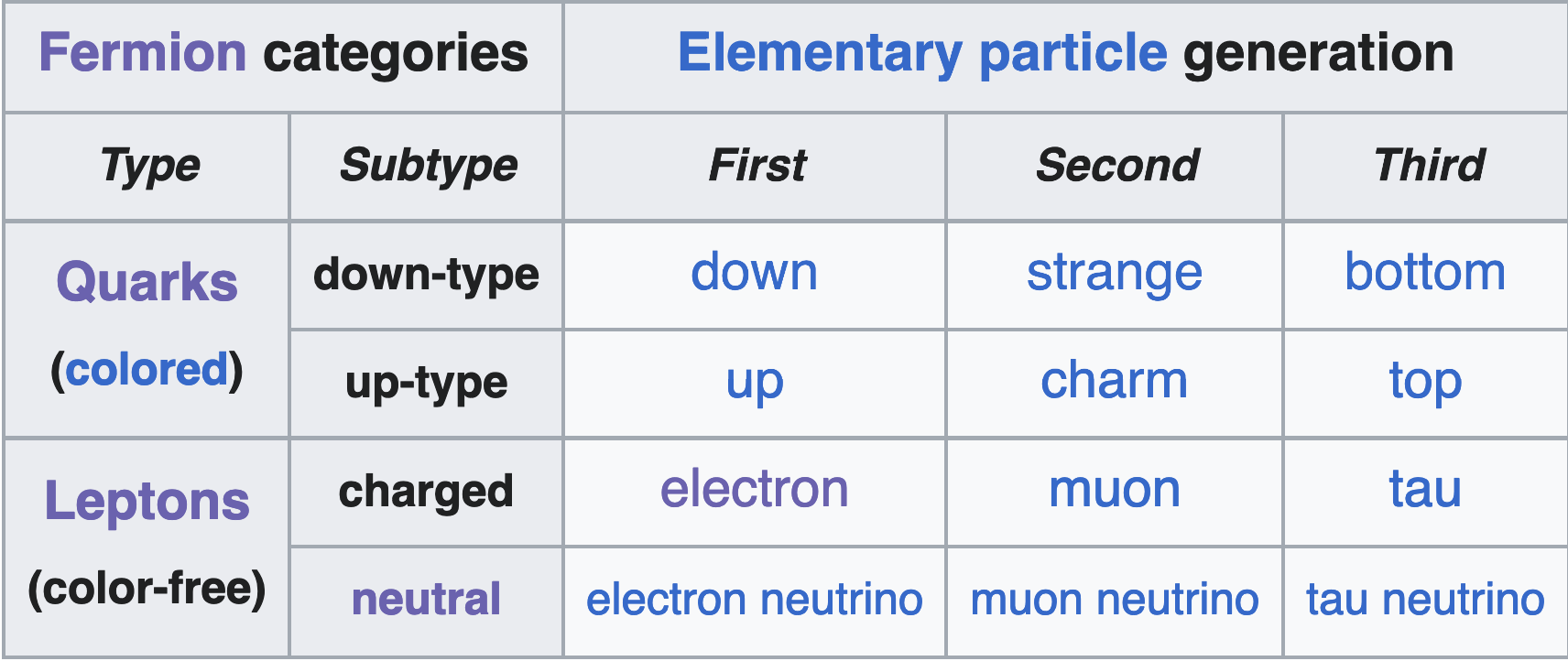
Bosons
| Type | Mass | Spin | Charge | Force carrier | Notes | Notes on carrier |
|---|---|---|---|---|---|---|
| (photon) | 0 | 0 | Electromagnetic (interacts w/ charge) | Massless, only can't be 0. | ||
| (gluon) | 0 | 0 | Strong force | Ditto above | Strong charge is a complex 3-vector , each component "color charge" red/blue/green. | |
| bosons | 100 GeV | W: Z: | Weak force | |||
| Graviton | Gravity (relativistic energy) | Not found yet | ||||
| Higgs | 125 GeV | Higgs field | Particle mass is charge, insignificant compared to others. |
- These are the force carriers which cover fundamental forces.
- Photons and gluons are their own antiparticles.
Conservations
- Energy, momentum, and angular momentum are all conserved
- Spin on right can be different by integer 1s, but not by .
- Total electric charge
- Lepton number (number of leptons + antileptons)
- Lepton flavor (electron-ness, muon-ness, tau-ness conserved, except for neutrinos)
- Opposite neutrino if creation, same neutrino if decay.
- Whenever neutrinos are produced, weak force
- Weak force ignores this idea
- Baryon number (quarks + antiquarks in composite particles)
- Quark flavor (conservation of quark type)
- "Similarly, the only way for the strong or electromagnetic to get rid of a strange quark is to annihilate it with an anti-strange quark"
- Violated by weak force
Complex particles
Baryons: 3x quarks, Mesons: 1 quark, 1 antiquark, Antibaryons: 3x antiquarks,
- Leptons have baryon number of zero (not composed of quarks)
- Same with bosons
Which interaction?
- Short lifetimes (), only hadrons and composite particles likely strong force.
- Flavor conserved.
- Medium lifetimes , photons involved, likely electromagnetic.
- Flavor conserved.
- Long lifetimes , results include neutrinos and leptons, likely weak force
- Flavor violation allowed.
Group theory
In mathematics, a group is a set with an operation that combines any two elements of the set to produce a third element within the same set and the following conditions must hold.
- : general linear group, all invertible matrices
- : unitary group, all matrices such that
- : belong to and have
- : belong to , only made with real numbers
- : belong to and have unit determinant
Misc
Matrix-vector mult:
Commutator of two operators is
- If zero, share same eigenvalues
is the "rest length", is the "rest time".
Finding eigenstuff
Eigenvalues:
Eigenvectors:
eigenvalue, corresponding eigenvector
Quantum stuff
is the spin (angular momentum) quantum number, is the spin component quantum number.
Operator
For example:
Chapter 8 - Ordinary Differential Equations
Reference "Mathematical Methods in the Physical Sciences" 3e by Mary L. Boas.
Differential equations are equations that contain both a function and it's derivative. Partial differential equations contain partial derivatives: If there are no partial derivatives, it's an ordinary differential equation. Some properties:
- Order is the highest derivative in the equation (i.e. is second-order).
- Linear equations will take the form where and are constants or functions of the independent variable (), but not of the dependent variable (). is nonlinear.
- Solutions usually mean to solve for the dependent variable: i.e. .
A linear differential equation of order will have a solution (the general solution) containing independent constants , from which all solutions of the diffeq. can be found by changing the values of the independent constants .
The values of these constants can be found using boundary conditions or initial conditions (at ).
Separable Equations
Separable differential equations are those for which we can separate the variables, putting the dependent variable on one side, independent on the other: The general solution will often have some form which represents a family of solutions (by varying ). A particular solution is therefore some single value of .
Nonlinear equations
Separable equations may also be nonlinear, such as Solving it as a separable equation yields which allows for only non-negative solutions for , and is not valid for ( for is undefined).
First-Order Equations & Int. Factor
Linear first-order ODEs take the form and are most easily solved via an integrating factor.
- Let
- Write the equation as
- Integrate and solve for .
Nonlinear First-Order Equations
There are other methods to solve specific (but not all) first order equations.
Bernoulli equation: for equations of the form
- Let:
- Multiply both sides by :
- Substitute in and :
- Solve for with integrating factor.
- Substitute (again) and find .
Exact equation: exact differentials (or "perfect" differentials) of some function (even an unknown one) have the property Integrals over them are path-independent.
- Let some function exist, such that
- By the definition of exact differentials, , and
TODO: Review chapter 6, section 8 for more information on finding .
Homogenous equation: a homogenous function of and of degree is one that can be written i.e. is homogenous of degree 3.
The equation where and are same-degree homogenous functions, is also homogenous. Dividing them cancels the terms as in the definition.
- Write
- Make the change of variable , such that
- Solve the resulting separable equation in and .
- Reverse-substitute to solve for .
Constant-Coefficient SOLDEs (Homogenous)
Second-order linear differential equations (or SOLDEs) with constant coefficients tend to look like and are homogenous if . They are solved using the differential operator , such that Solve for the roots as a second-order polynomial. Solutions vary based on multiplicity and complexity.
- If the roots are real and distinct ():
- If the roots are real and have multiplicity of 2 (i.e. ):
- If the roots are imaginary (): (I tend to use the second solution (5) - it's easiest and simplest).
Oscillators
Hooke's law + Newton's 2nd say that, for some simple harmonic oscillator, where is the spring constant and is the "retarding force".
Let and . This turns into The roots to the differential operator are , with three scenarios for answers:
Overdamped: is real and has two distinct solutions, so
Critically damped: , so real roots with one distinct solution.
Underdamped: , so imaginary roots
Method of Undetermined Coefficients
Non-homogenous constant-coefficient second-order linear differential equations The general solution to this equation is the sum of the homogenous and particular solutions: The particular solution can be found primarily through the method of undetermined coefficients.
- Let take the form of one of the solutions below, based on what looks like.
- Calculate and .
- Substitute in the guesses into the diffeq, then solve for the constants.
The textbook provides some additional solution options for equations of the form , where is some polynomial of degree .
Note: if there are several terms on the right-hand-size, we can use superposition with each term to find .
Other Second-Order Equations
Some other special second-order equations with methods to solve them are shown below.
(a). Missing dependent variable If is missing from the equation, substitute and . Solve for , then reverse-substitute and solve the first order equation for .
(b). Missing independent variable If is missing, let (c). . Multiply by , then integrate to get (d). Cauchy/Euler equations if equation has the form can be reduced to SOLDE C.C. by substituting to get (e). Reduction of order to find a second solution of given one solution , substitute into the differential equation and solve for .
Laplace Transforms
Laplace transforms are way to solve differential equations - for some function ,
For example, if , . This can be converted back into the original function by referencing a Laplace transform table.
Paul's Math Notes (of course) has a wonderful table here.
To use it,
- Apply the Laplace transform to all terms in the differential equation (both left and right).
- Plug in initial conditions.
- Group (or ) terms and try to isolate terms on each side (all terms on one side, terms on the other).
- Use table to find inverse Laplace transform of .
- If there isn't an exact equivalent on the table, try using partial fraction decomposition or other techniques to separate into individual terms, and sum them.
For higher orders of differential equations, plug into and use integration by parts.
Dirac Delta Functions
The Dirac delta function lets us model functions which change rapidly over a very short () period of time, such as unit impulses (a hammer strike, or the impact of an air particle).
 at is mathematically infinite - not very useful at all. Instead, we can represent this increase by a delta function:
This is a generalized function, with the following properties:
at is mathematically infinite - not very useful at all. Instead, we can represent this increase by a delta function:
This is a generalized function, with the following properties:
- Derivatives of the function turn into derivatives of :
- is an operator. Let .
Some other properties: can also work in two and three dimensions, and vectors:
Finally, in three dimensions we have two useful operator equations:
Green's Function
I'm not confident in my knowledge of these - Boas 8.12 has more info on them, but the presented examples seem surprisingly complicated.
As far as I can tell, just as for there is some (for invertible matrices) such that , is a similar transform for differential equations such that - see this Stack Exchange post.
The Wikipedia page on Green's function says that, if is some differential operator, then
- is the solution of the equation .
- The solution of the IVP is the convolution .
From Boas: for some differential equation , we can represent as a sum of unit impulses: For instance, if models the air resistance on some oscillator, a unit impulse might be a single air particle bouncing off the oscillating object.
The differential equation in terms of unit impulses can be written with being a differential operator (like or ): and the solution is
The example on the Wikipedia page for Green's function provides (in my belief) a much better explanation than Boas does.
Chapter 11 - Special Functions
Reference Mathematical Methods in the Physical Sciences (3e) by Mary L. Boas.
Factorial functions
Factorial functions are defined as More memorably, factorials are the product of their sums: A table of the initial ones is below.
| 0 | 1 |
| 1 | 1 |
| 2 | 2 |
| 3 | 6 |
| 4 | 24 |
| 5 | 120 |
Gamma functions
For any , The is further easily defined in terms of factorials: Useful is also the recursion relation:
The gamma function seems useful for working with both fractions and complex numbers.
For negative numbers where , Also, some special formulae: Note: this last equation is undefined for integer
Beta functions
Beta functions, I'm not sure what they're useful for. But Boas gives several representations of it, which I'll include below.
For :
Also, note that .
In terms of gamma functions,
Chapter 14 - Functions of Complex Variables
Reference "Mathematical Methods in the Physical Sciences" 3e by Mary L. Boas.
We can represent a complex function (those including ) by :
Or, alternatively, with and :
 Complex functions are those that are a function of :
and are composed of their real and imaginary parts, represented by and :
Complex functions are those that are a function of :
and are composed of their real and imaginary parts, represented by and :
Note: is customarily single-valued (one unique value per ). To handle functions that aren't single-valued (), define a range such that or or are permitted.
Analytic Functions
A function is analytic in a region of the complex plane if it has a unique derivative at every point of the region.
Similarly, the statement " is analytic at some point " means there's a unique derivative in some small circle around .
For some analytic function , the derivative is defined as where . Note also some definitions:
- A regular point of is a point at which is analytic.
- A singular point / singularity of is a point at which is not analytic.
- This is an isolated singular point if analytic everywhere else in a small circle around .
Ex. derivative of an analytic function: .
Ex. derivative of a non-analytic function: Using our limit idea above, the numerator is always real (abs. values always real), but the denominator has different values depending on the approach. It's neither always real nor purely imaginary.
Thus, is not analytic.
Some relevant theorems about analytic functions:
Theorem I: if is analytic in a region, then in the region these are the Cauchy-Riemann conditions.
Theorem II: if and (and their partial derivatives w.r.t. and ) are both:
- Continuous.
- Satisfy the Cauchy-Riemann conditions.
Then is analytic at all points in the region (though not necessarily the boundary).
Theorem III: If analytic in a region, then it has derivatives of all orders at points inside the region, and can be expanded in a Taylor series around any point inside the region.
The power series converges inside the circle around which has a radius until the nearest singular point.
Theorem IV: If is analytic in a region, then and satisfy Laplace's equation in the region (i.e. and are harmonic functions).
Also, if or satisfy Laplace's equation in a simply-connected region, they are respectfully the real or imaginary parts of an analytic function .
Note: this means we can find solutions of Laplace's equation just by taking the real or imaginary parts of an analytic function of .
Contour Integrals
Some additional theorems of analytic functions involve contour integrals - or path integrals in the complex plane.
Theorem V (Cauchy's theorem): If is some closed, smooth curve (corners allowed) in the complex plane, and is analytic on and inside , then Note: a finite number of corners are allowed.
Theorem VI (Cauchy integrals): if is analytic on and inside some closed curve , then inside is given by the path integral along below: If is given on the boundary of a region (), then this integral gives the value of at any point within .
Laurent Series
Laurent series are able to represent complex functions as power series, which include terms of negative degrees.
Theorem VII (Laurent's theorem): Let and be two circles centered at , and analytic in the region between the circles. can be expanded as convergent in . The terms are called the principal part.
Some properties of :
- If all , is analytic at and is a regular point (see Analytic Functions).
- If but all terms after , has a "pole of order" at . If (i.e. , ), has a "simple pole".
- If all , has an "essential singularity" at .
- The coefficient is the "residue" of at .
Residue Theorem
Fourier Transforms
Chapter 7.12 in "Mathematical Methods in the Physical Sciences" 3e by Mary L. Boas.
These are so cool. Go check out the Falstad Fourier applet.
Fourier series are useful for visualizing periodic functions as a sum of discrete coefficients and sines/cosines.
Visually, this GIF from the Wikipedia article on Fourier series is delightful.
Fourier integrals on the other hand are useful for representing both nonperiodic and periodic functions in terms of sines and cosines.
Let be the function and its Fourier coefficients. The associated Fourier transforms are
Though these are in terms of , we can convert them using Euler's formula:
To solve them,
- Plug the original function into the equation.
- Solve for .
- Solve for the Fourier transform.
Cosine and sine transforms
We can use cosine and sine transformations to represent even and odd functions respectively to simplify the calculation of Fourier integrals.

Cosine Transform: if is an even function where ,
Sine Transform: if is an odd function where ,
Chapter 1 - Stern-Gerlach Experiments
Reference Quantum Mechanics: A Paradigms Approach by David McIntyre.
First conceptualized in 1922 by Otto Stern and later performed by Walther Gerlach, the SG experiment involved sending a beam of silver atoms through a nonuniform magnetic field and observing their distribution.

Classically, the distribution ought to look like the input beam - since silver atoms are electrically neutral, the nonuniform magnetic field shouldn't affect them, and they should just pass through.
Experimentally, we see the silver beam split at the magnetic field into roughly equal-sized groups, indicating not only that the magnetic field interacts with the silver atoms, but that each electrically-neutral silver atom must have some additional property that interacts with a -field (i.e. that the -field puts some force on the silver atoms based on some binary property).
We know (ref: Wikipedia entry on magnetic fields), where is the magnetic moment and is the magnetic field strength. Classically, should be zero for a neutral atom (all atoms hit the center) - however, we see that there must be forces on the atom since our atoms diverge from the beam at the -field. Further, we have an "upper" and "lower" group with equal distances - so . With known to be constant, then by the results of the experiment we must have two values for : and (the magnetic moment values are quantized).
Enter: Electron Spin
If we imagine (classically) an electron as a charge moving around a loop of current,

then . Here, and , so Thus, (classically), we can imagine each charge as having some "orbital angular momentum" (like planets around a star). Angular momentum is , so we can rewrite this as Experimentally, we observe that, while normal orbital angular momentum of charged particles still "exists", it's not the whole picture - we also need "spin", where we can write as where is a dimensionless "gyroscopic ratio" (note: different from planet spin since electron is almost a 1d point). For an electron in the direction, and, to achieve the results we observe in the experiment, we can have only two values of : where is a modified Planck's constant . This binary value represents a spin-1/2 system, though these aren't the only two possible values.
Quantum States
Postulate 1: the state of a quantum mechanical system includes all information we can know about it. Mathematically, we represent this state by a "ket", .
In the spin-1/2 system,
where is the quantum state of the atoms that are spin-up , and is the quantum state of the spin-down atoms .

Stern-Gerlach ran a few experiments using this basic setup to get a better understanding of the quantum nature of spin, and explore this divergence from what is classically expected.
-
Experiment 1: Analyzing spin in twice in a row. Spin values were conserved between measurements - if we only take atoms and measure again, we only see atoms.

-
Experiment 2: Analyze spin in , then in - was found to be totally independent whether we used or .
 Complicated, though - this is a mixed state, rather than the superposition of experiment 1. We'll investigate options to make it nicer later.
 -
Experiment 3: Analyze spin in , then , then . We expected to see the spin values conserved - but don't! Instead, by measuring , we find we "reset" the spin of .

-
Experiment 4: Analyze spin in , then , then - however, instead of measuring , just send both outputs into the next . Somehow, by not "measuring" , we don't reset the spin measurement.

Bra-ket notation
Used to represent quantum state vectors, which lie in the Hilbert vector space. The dimension of the Hilbert space is determined by the current system - in our above example, we have only two possible results, so represents a complete basis with dimensionality 2.
Note: and are complex scalar multiples. Some properties of the bra-ket notation (Dirac's first and only pun):
- Each ket has a corresponding bra, such that for some state ,
- Multiplying a bra with a ket represents an inner (dot) product.
This means we can multiply with to get each constant (i.e. here), such that
Likewise, and .
- All quantum state vectors must be normalized, such that
If we wanted to normalize some vector , apply some normalization constant , such that and solve for .
Note: will be an absval by the end here - but we don't care about it's phase (not physically meaningful), so just make it real and positive.
- The complex constants and when squared (i.e. ) represent probabilities for a given measurement (probability for or above). The normalization property implies the probabilities must sum up to 1 - helping prove postulate 1.
Matrix form
We can also represent states in matrix form, where and with the corresponding bra represented by the row vector so
General quantum systems
For some general quantum system, where we might not only have 2 results (i.e. not only spin-1/2), such as

then, generally speaking,
Note: represents each corresponding complex scalar multiple, and is the Kronecker delta, which is 1 if and 0 if .
Converting kets between axes
We can represent up-down spin measurements in and in terms of our -spin kets, such that
In matrix form,
The Postulates of Quantum Mechanics
Postulate 1: the state of a quantum mechanical system, , contains everything we can mathematically know about it - experimentally, the hidden variables theory (regardless of validity) is irrelevant (since the variables are by definition hidden.)
Postulate 2: Physical observables (such as spin) are represented mathematically by some operator that operates on kets.
Postulate 3: The only results possible from a measurement are contained in the set of eigenvalues of the operator .
Postulate 4: The possibility of obtaining some eigenvalue in a measurement of the observable on the system is g
Postulate 5: After a measurement of (such as spin) that yields some result (such as ), the quantum system is in a new state that is a normalized projection of the original system ket onto the ket (or kets) corresponding to the result of the measurement
Postulate 6: The time evolution of a quantum system is determined by the Hamiltonian, or total energy operator via the Schrödinger equation
Note: only postulates 1 and 2 were covered in this chapter.
Chapter 2 - Operators & Measurement
Reference Quantum Mechanics: A Paradigms Approach by David McIntyre.
Operators are mathematical objects that operate on kets to turn them into new kets; is one such example. If a ket is not changed by the application of some operator, then the ket is known as an eigenvector and the associated constants are eigenvalues. Above, is the eigenvector and is an eigenvalue. Both eigenvectors and eigenvalues are properties of the operator - if it changes, so does the eigenstuff. For the operator , the eigenvectors / values are:
Postulate 3: The only possible result of a measurement of an observable (like ) is one of the eigenvalues of the corresponding operator .
This postulate implies that, if we have the eigenvectors and values of , we can actually reconstruct from them.
Let . Which leads us to Now, plugging these solved values in,
- Operators are diagonal in their own basis (i.e. they only have elements along the main diagonal).
- The elements along the diagonal are the eigenvalues of the operator.
- The eigenvectors themselves are not included in the operator matrix.
Note: an observable is some physical quantity that can be measured - such as spin. In that context, the operator represents that observable.
Other representations of matrix elements
We can also represent an operator matrix in terms of its elements. Let the operator describe some two-dimensional spin-1/2 system (like does).
Where
Finding eigenvectors / values from an observable
If we know the operator , and need to find the possible results of a measurement of the corresponding observable, we can start from the general eigenvalue equation and work from there.
where is the eigenvalue and is the corresponding eigenvector. Eigenvalues can be found then by solving the secular equation, Note: for a operator (i.e. a spin-1/2 system), this is .
After finding the eigenvalues, we now know and - all that remains is to find by solving for it in .
The process of finding the eigenvectors and eigenvalues of a matrix is known as diagonalization.
Hermitian operators
To find the associated bra operator to some operator acting on a ket, we use the operator
where is the Hermitian adjoint of , found by transposing and taking the complex conjugate of . If , then is said to be Hermitian, and for .
This is not normally the case - if is not Hermitian, the corresponding bra-state operator will be different from - i.e. will not be the bra corresponding to .
Hermitian operators have some properties to be aware of:
- They will always have real eigenvalues which ensures the results from a measurement are always real.
- The eigenvectors of a Hermitian operator form a complete set of basis states, ensuring we can use the eigenvectors of any observable as a valid basis.
New operators
Let's say we wanted to find the spin component in some general direction .
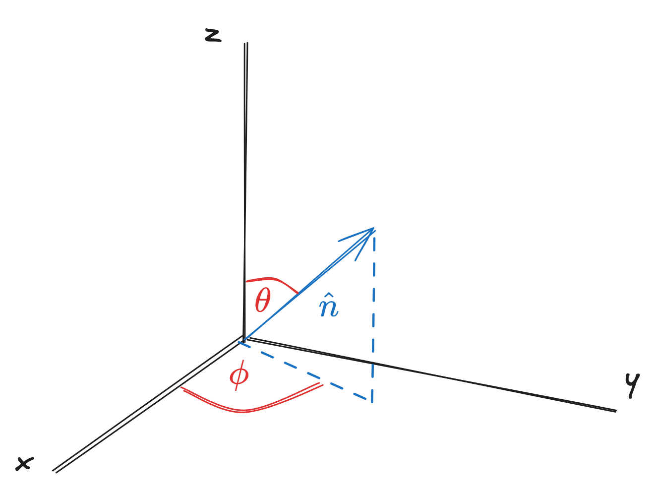 where . Projecting the spin vector onto such that
then
and diagonalizing the vector above, we find the eigenvectors for to be
with the state vector
where . Projecting the spin vector onto such that
then
and diagonalizing the vector above, we find the eigenvectors for to be
with the state vector
Note: the coefficient calculation attached to is from total probability being equal to 1.
Outer product
Instead of taking the inner product between two state vectors, we can also find the outer product (). For example, we can rewrite as and are called projection operators:
This last formula is known as a closure or completeness relation due to the equivalency to the identity operator , meaning that these basis states form a complete set of states.
When our projection operator acts on some state ,
Note: is equivalently the or coefficients.
and the probability of observing some state is then This allows us to write the fifth postulate
Postulate 5: After a measurement of some observable operator that yields the result , the quantum system is in a new state that is the normalized projection of the original system ket onto the new ket corresponding to the result of the measurement
Returning to Stern-Gerlach 3 & 4
We were able to look at experiments 1 and partially 2 in chapter 1, but not experiments 3 and 4, which required expounding on operator products a bit further.
Experiment 3
Experiment 3 measured , then measured , then again, observing a "reset" with the other measurement.
The probability that an atom stays throughout the three measurements is the product of each probability - such that
Likewise for it to be , then , then is
Tradition holds QM magnitudes / probabilities to be read from right to left.
Experiment 4
Experiment 4 measured , then put the atoms through an analyzer (but didn't measure them), then measured again, finding the "measurement" step to be an important one.
The results in this one are interesting but simple - representing them with postulate 5,
This can be expanded out (and is done so in McIntyre 2.2.4), but will not be included here for the sake of brevity.
Mean and Standard Deviation
The expected mean (or expectation value) of some measurement is represented by , such that and is a sum of each possible result multiplied by the probability of that result.
Probability can be represented by both outer products and inner products - inner products are more readable, but require squared absvals , while outer products require more terms overall.
We can also write the expectation value for some operator as For , this can be written out as
Which makes sense, given is the only possible result of a measurement of for the state. For some system prepared .
Standard Deviation
The root-mean-square deviation (r.m.s. deviation) is
In the rightmost version, the second term is the squared expectation value. The first term, in the case of the initial state, can be expanded into and Expected, since we only have one possible result for measuring - so no spread of possible results.
Commuting Observables
Note: eigenstates are equivalent to eigenvectors.
The commutator for two operators is defined as If the commutator is zero, then the two operators (observables) commute. If nonzero, they don't commute. Logical consequences can be determined by just this statement alone - the first being: The order of operation doesn't matter for commuting observables. Now, let be an eigenstate (eigenvector) for some operator with eigenvalue : Let's apply to both sides of this. Using the commutability of and , This last equation says is also an eigenvector of corresponding to the same eigenvalue . Thus, must be a scalar multiple of (let's say this scalar multiple is ) - and we can write Commuting operators will therefore share common eigenvectors - this means the two operators (that represent observables) are compatible, and we can measure one without erasing our knowledge of the results of the other observable.
This is often phrased as knowing the results of these observables simultaneously, though realistically we're still measuring each sequentially.
If two operators do not commute, then they are incompatible. This is the case for our orthogonal spin operators - and the commutations for , and are
The Uncertainty Principle
We can relate the product of two standard deviations (i.e. uncertainties) of two observables with the commutator by
The Uncertainty Principle: the product of two uncertainties will always be greater than or equal to the absolute expected value of the two.
For the and spin components,
Implying and - while we can know one spin component, we can never know the other two (they are incompatible observables).
Operator
and is represented in matrix form as
Thus, since the operator is proportional to the identity operator, it must therefore commute with all the other operators and - this implies all states are eigenstates of the operator, and we can write for any state in the spin-1/2 system. The vector has an expectation value of
and a "length" of
This is longer than the "normal" measured component of along any axis - implying the spin vector can never be fully aligned along any one axis, since there will be always components in other axes.
This is often called "quantum fuzziness".
Regarding Photons
Photons also have spin - but due to moving at (ultra-relativistic), it can never have a spin of 0 - must be either .
Spin-1 Systems
Fermions are particles with spins of multiples of 1/2 (i.e. , , ), while bosons are those with full-integer spins (i.e. , , ). Spin-1 bosons have spin states of , or
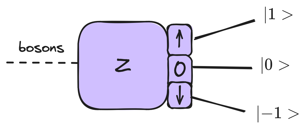 where
where
The eigenvalues , and are on the main diagonal of .
For ,
and for ,
Note: The Stern-Gerlach experiments have conceptually the same results - but note that experiment 2 differs (not all 1/3 - rather, one is 1/2, the other two 1/4).
General Quantum Systems
Let denote the spin of some -spin system with number of beams (i.e. for a spin-1 system, this would be 3, spin-1/2 system, 2). Let the possible values for spin on the axis be labeled by - then,
is known as the spin (angular momentum) quantum number and is the spin component quantum number (or magnetic quantum number).
In spin-1/2, and in spin-1,
Chapter 3 - Schrödinger Time Evolution
Reference Quantum Mechanics: A Paradigms Approach by David McIntyre.
The time evolution of a quantum system is governed by the differential equation
where corresponds to the total energy of the system (the Hamiltonian operator, different from the Hermitian operator - though the Hamiltonian is still a Hermitian operator).
Postulate 6 The time evolution of a quantum system is determined by the Hamiltonian (total energy operator) , through the Schrödinger equation:
The eigenvalues of the Hamiltonian are the allowed energies of the quantum system, and the eigenvectors (eigenstates) are the energy eigenvectors of the system, such that
The Energy Basis
Let's say we've already diagonalized and found values for the allowed energies and . General state vectors can be written in terms of these energy eigenstates: and, since the energy eigenvectors are orthonormal, we can write the energy basis as Assuming the Hamiltonian in this context is time-independent, such that for all , then the time-dependent Schrödinger equation can be written where , an angular frequency.
Stationary States
Let's start with the simplest possible situation, where the quantum system is in one single energy eigenstate: After some time , this system will be in the state where . This state, however, differs from our initial state only by the phase factor , and since phase changes will never affect the probability of measurements, the probability of observing some eigenvalue for an observable will be This probability is time-independent and equal to the probability at . There is no measurable time evolution for this state, and the energy eigenstates are called stationary states - if a system begins in some energy eigenstate, it will remain in that state.
This same idea goes for multiple energy eigenstates: where
Non-commuting Observables
If an observable commutes with , then and have common eigenstates - so measuring is equivalent to measuring . However, if does not commute with , then the two observables will not share common eigenstates, and the eigenvalues of will be some superposition of energy eigenstates.
Let the eigenstates of corresponding to be represented by and the probability of measuring would be The overall phase drops out - only the relative phase between and remains. which is the also Bohr frequency.
Summary
In a time-dependent quantum system with a time independent Hamiltonian , the probability of measuring of some observable at time can be found through the following process:
- Diagonalize to find the eigenvalues and eigenvectors .
- Write in terms of the energy eigenstates .
- Multiply each eigenvector coefficient by to get for some arbitrary .
- Calculate the probability .
Time Evolution of Spin
Let's apply Schrödinger time evolution to the spin-1/2 system.
The Hamiltonian operator represents the total energy of a system. In time-dependent solutions, only energy differences are important - thus, the Hamiltonian is just the magnetic potential energy of a spin system If we say the gyromagnetic ratio and (an electron), then
-direction
In the direction, , and
where , and
with eigenstuff Applying the Schrödinger time evolution to a general state in direction with phase shift in : If we were to calculate the probability of measuring along the axis for this arbitrary direction and phase ,
Probability here is time-independent because the eigenstates are also energy eigenstates for this problem (i.e. and commute).
-direction
The probability of measuring spin along the direction instead, where instead of we have is:
Probability in the axis is time-dependent because the operator does not commute with .
For -direction, we'd use the same equation as above, except with instead.
Expectation values
Irrespective of the three axis is the total spin vector's expectation value , the precession of which is known as Larmor precession, with frequency known as the Larmor frequency. The expectation value of the spin vector precesses in a uniform magnetic field, as visualized below.

Ehrenfest's theorem states that quantum mechanical expectation values obey classical laws - as visualized above, the precession of the spin vector makes it clear the system has nonzero angular momentum (as opposed to just a magnetic dipole moment).
Magnetic field in a general direction
Let's say we have a magnetic field with both an and component, such that This field will be oriented in the -plane with some angle w.r.t the -axis. First, we'll define Larmor frequencies with each field component: And the Hamiltonian is then defined as This Hamiltonian isn't diagonal - so we need to diagonalize it. This leads to
When , the energy eigenvalues are just , same as .
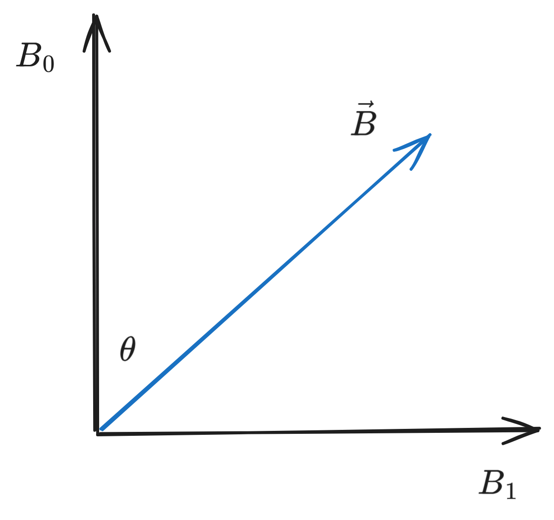 From the above figure, we know
and
where is the spin operator in some direction , with vectors (found in chapter 2)
From the above figure, we know
and
where is the spin operator in some direction , with vectors (found in chapter 2)
Spin flip
The probability that some initial state later evolves into (known as spin flip) is
This is called Rabi's formula - see the Rabi cycle.
Neutrino Oscillations
Neutrinos are produced via decay processes, such as where is an electron neutrino and is an electron antineutrino. Neutrinos interact with normal matter via the weak nuclear force (the weakest of the four fundamental forces), making them extremely hard to detect. Other flavors of neutrinos are produced via processes such as the pion-muon decay and muon-electron decay: where is a muon electron.
Electrons, muons and tau () particles, as well as their neutrino byproducts, are known as leptons.
There is no theoretical basis for conservation of lepton flavors, so reactions of the type are possible, where an electron neutrino changes flavor to a muon neutrino or visa versa - these reactions are known as neutrino mixing or neutrino oscillations.
When neutrinos are interacting with the weak nuclear force, they have some energy within that interaction, and the quantum states and are eigenstates of the Hamiltonian describing the weak nuclear force - in free space, with no weak nuclear force present, the only relevant Hamiltonian (energy description operator) is the relativistic energy of the particle (which due to includes the rest masses and momenta) - this relativistic Hamiltonian has mass eigenstates.
If , then the mass eigenstates do not coincide with the weak interaction eigenstates - allowing for flavor-changing processes in the first place (somehow?).
Let where is the mixing angle between the two. If this angle is small, then the small angle hypothesis applies and
Example
Assume an electron is created by a weak-interaction process and propagates through free space to a detector. We detect it by seeing the signature of flavor mixing, rather than the neutrino itself. Let our initial neutrino be an electron neutrino: Since this neutrino's now propagating through free space, the energy eigenstates are just its mass eigenstates (no weak interaction) - so the Schrödinger time evolution is where represents the relativistic energy eigenvalues, determined by the rest mass and momenta of each. Assuming the neutrinos are highly relativistic, then and The probability of the neutrino mixing is The energy difference is just proportional to the difference in masses (see above), and, with where is the distance from the source from the detector and momentum : The probability oscillates from 0 to a maximum value of ... hence the term neutrino oscillation.
Experimental measurements have this mass difference is approximately and .
Time-dependent Hamiltonians
Thus far, we've only looked at time-independent Hamiltonians. Time-dependent Hamiltonians are to them what a salmon in the ocean is to nigiri - complicated.
Generalizing Rabi's formula with the change , where is the frequency of incident light (i.e. incident light is not static, but oscillates with time). For the case of (zero-frequency light), the applied field is static and we can use our earlier definition of Rabi's equation.
The static field case () is referred to as spin procession, the rotating field case () as Rabi flopping. In the static field case, the spin precession is a natural oscillation of a quantum system operating in a superposition of energy eigenstates. In the rotating field case, the Rabi flopping represents transitions between energy eigenstates, and there is an exchange of energy between the particle system and the applied rotating field - since the Hamiltonian is time-dependent, energy is not static within the system, but moving into and out of the applied field.
Time-dependent Hamiltonian
Let's look at the scenario where some incident photons collide with some matter, increasing the energy levels of local electrons.
In a quantum sense, the oscillating electric field of the light wave interacts with the electric dipole of the atom, and the energy exchange between the field and the atom corresponds to the absorption and emission of photons.
The probability of a Rabi spin flip changes/oscillates with the angular frequency (typically referred to as the generalized Rabi frequency - though the Rabi frequency itself usually refers to .
The Hamiltonian of this system is
Resonant frequency
If , the frequency of the rotating field is equal to the Larmor precession frequency , and the probability of a spin flip just becomes
Spin is flipped with 100% probability with some frequency .
Non-resonant frequency
At values , the spin flip oscillates with an amplitude smaller than 1.
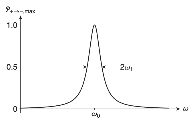
The FWHM of the above curve is .
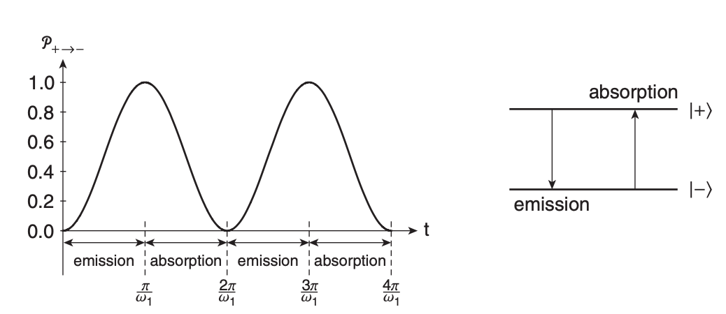
Chapter 4 - Quantum Spookiness
Reference Quantum Mechanics: A Paradigms Approach by David McIntyre.
In the 20th century, as quantum mechanics was first developing widespread acknowledgement, various theories were put forth to try and explain the probabilistic (rather than deterministic) nature that surprised a lot of classical physicists.
Einstein-Podolsky-Rosen Paradox (EPR)
Some, such as Albert "God does not play dice" Einstein, thought the probabilistic nature of QM (especially when juxtaposed with the more-deterministic classical mechanics) was just because we weren't seeing some variables - we thought it probabilistic only because there was some backstage action we weren't seeing (an incomplete description of reality).
The experiment begins with an unstable particle with spin 0, which then decays into two spin particles (consv. of angular momentum) traveling in opposite directions (consv. of linear momentum).
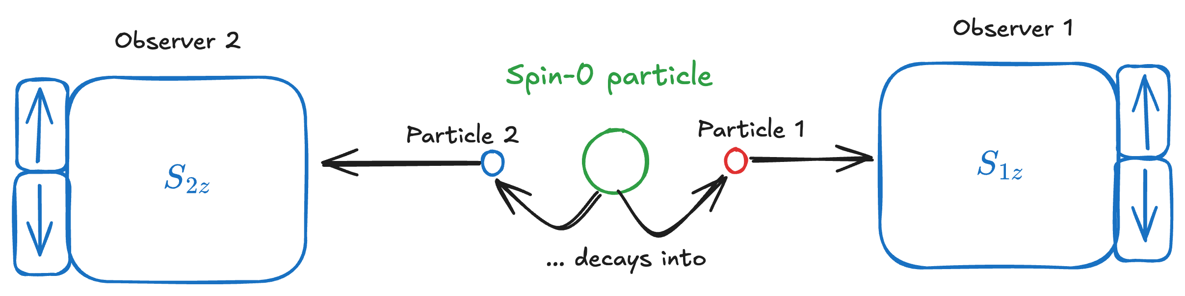
Because each spin is opposite the other, if observer 1 sees spin +1/2, observer 2 must see spin -1/2, and visa versa. After measurement, each observer always knows what the other observer sees.
This would be later called an entangled state.
There are two ways of looking at these particles:
- Each exists as part of a state that is in superposition, so neither particle has a defined spin until measurement.
- Both particles have spin values defined at the moment of decay - particle 1 always had spin , particle 2 always spin .
For example, imagine a particle decays on Earth, and the resulting 1/2 particles are kept (unmeasured) in two chambers (i.e. the quantum state describing both is in superposition by view 1). One 1/2 particle is sent with a ship to Mars, and another is sent on a ship to Alpha Centauri.
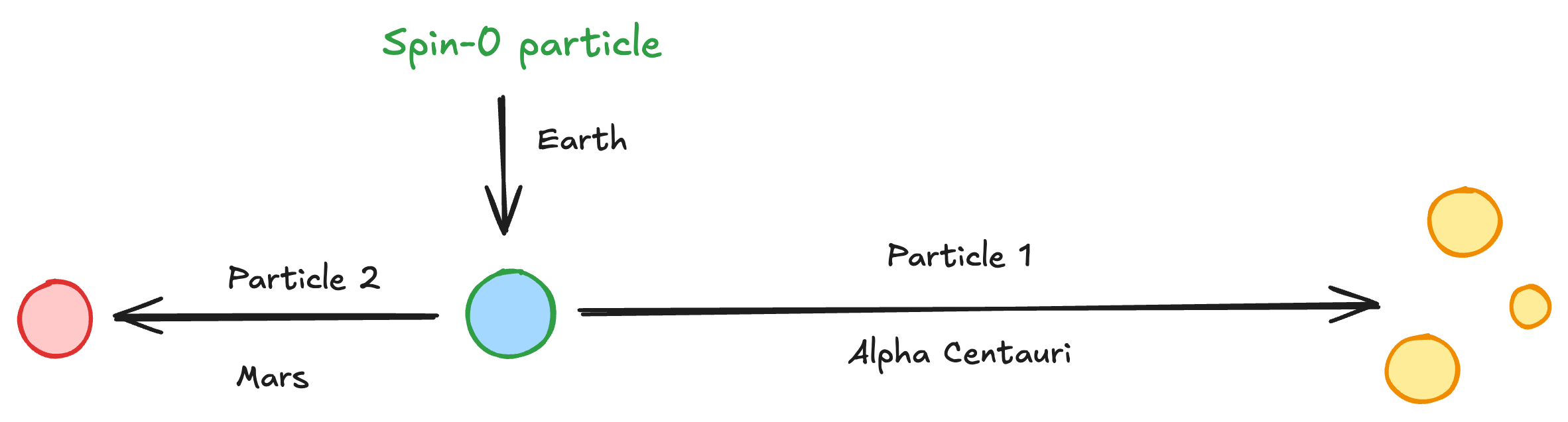 If Mars makes the measurement , according to idea 1, the state instantaneously collapses into the state and Alpha Centauri will measure , regardless of the distance between the two. Idea 2 says that Mars always had , while perspective 1 maintains that the superposition state must have collapsed then.
The EPR paradox argues in favor of the second: the spin is a "real" property of the particle - a variable (invisible to our instruments then) describing reality. Instead of being in a superposition state pre-measurement, both particles had their spin states specified at the moment of decay and always did - Einstein's local hidden variables theory (localized to each particle).
For a while, it was thought impossible to know whether theory 1 or theory 2 was the correct interpretation ... that is, until 1964. Enter John Bell.
Bell's Theorem
Bell's theorem sets up a mathematical inequality that provides different results for a setup assuming HVT and a setup assuming the Copenhagen interpretation.
In the hidden variables theory (HVT) interpretation, this equality is where and represent the measurements taken by two observers and and denotes the expectation (or average) value of some measurement. This inequality is also called the Clauser-Horne-Shimony-Holt (CHSH) inequality.
Now, assume this was set up with qubits instead - see the Wikipedia article for more details. Summing the expectation values yields which is greater than the maximum of 2 allowed by the CHSH inequality, implying hidden variables cannot exist.
Schrödinger's Cat
Schrödinger, in a fit of psychosis, proposed putting a cat in a box. Never a good idea - but further, he decided that box should include both unstable radioactive isotopes and a bottle of cyanide! If an isotope decay is detected, boom. Dead cat.
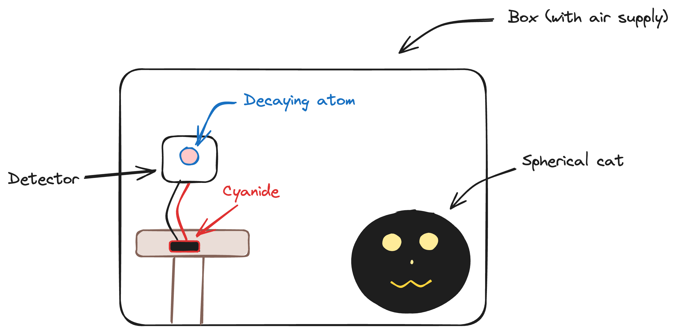 Now, this is a dumb experiment for so many reasons (animal cruelty not the least of which), but it's animal cruelty for science ... so ... yeah. That doesn't even justify it. Whatever. Don't do this experiment at home or anywhere else for that matter.
The atom has a half life of 1 hour. After 1 hour, the state of the life-deciding decaying atom is described by ... with the quantum state of the cat implied to be ... implying the cat is in a superposition state between dead and alive. Purgatory's got nothing on Schrödinger's pets. This (thankfully only) thought experiment raises two questions:
- Can macroscopic (cat) states be described quantum mechanically?
- What qualifies as a measurement? I.e. what causes the collapse of the wave function?
The Copenhagen interpretation states that, no, cats (nor any other macroscopic thing for that matter) cannot be represented by quantum functions - only classically, like with ... normal things, like what color it is, food, how fast it's going, etc. Normal things, like, by Jove, physicists are weird.
More human-centric folks have argued human consciousness causes the collapse, others that there is no collapse - rather, just a bifurcation into separate universes (the multiverse).
Feynman had the non-answer to answer this:
Shut up and calculate.
Chapter 5 - Quantized Energies
Reference Quantum Mechanics: A Paradigms Approach by David McIntyre.
Spectroscopy
Atoms are differentiated by their specific atomic structure - how many neutrons, protons and electrons they have form the basis for elements in the periodic table. Electrons form the bulk of ways we can identify one element from another - when an atom absorbs a photon, the atom responds by raising an electron up one energy level, then dropping it (emitting a photon).
Since the energy of a photon is and we can only have specific values of energies, we can identify individual atoms by their frequencies - i.e. with quantized values for energy come quantized values for frequencies.
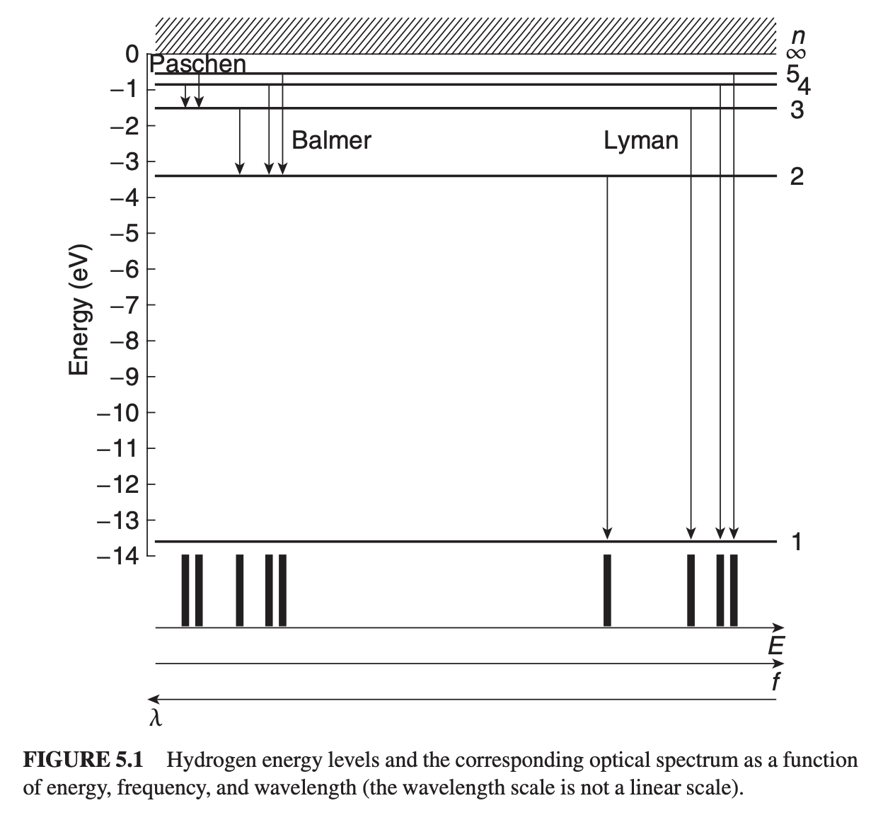
The lowest energy state ( for hydrogen) is called the ground state, with higher levels called excited states. The set of quantized energy states is referred to as the energy spectrum of a system.
From a quantum perspective, we can visualize the energy spectrum like this:
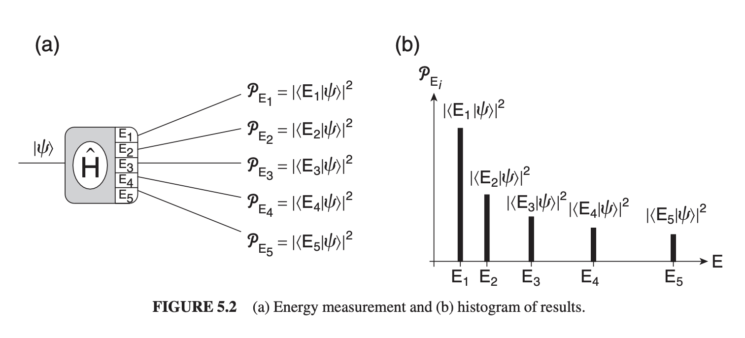
For a system prepared in some initial state , the probability of measuring some energy shift is We can find the energy levels and their corresponding eigenstates by applying the Hamiltonian in the energy eigenvalue equation, such that
Energy Eigenvalue Equation
Also known as the time-independent Schrödinger equation since it can be derived from the S.E. by separating the time and space components.
To find the equation describing energy eigenvalues,
- Find the classical form of the system's energy
- Replace each physical observable (position, momentum etc) with their quantum mechanical operators.
For a simple moving particle, the energy is the sum of kinetic and potential energy. where is the momentum of the particle in the direction and is the potential energy.
In quantum mechanics, our primary physical observables are usually position and momentum , so our energy operator is just the quantum version of using and : where is used to fix dimensions and ensure measurable results are real (non-imaginary).
Our quantum variables and are both used in wave functions, which are really just alternate representations of quantum states:
This is called position representation since we're using the position eigenstates as the preferred basis.
The wave function representing the energy eigenstates in position representation is so our energy eigenvalue equation becomes
Right. Let's combine everything. Using with our quantum variables: simplifying,
is the potential energy function, is the wave function representing energy and is the energy eigenvalue.
The big thing that happens with wave functions: operator equations turn into differential equations.
The Wave Function
The wave function is the probability amplitude for the quantum state to be measured in the position eigenstate , with the actual probability of measuring some value being

Probability density
Since the probabilities of all measurements still sum to unity, for a continuous probability density function , all of the following are equivalent:
Similarly, if we wanted to know the probability a particle would be found between and ,

Note: the above curves of represent probability density: By multiplying by , we get rid of the unit length and end up with probability.
Generally, to translate bra-ket formulae to wave function versions:
- Replace kets with wave function
- Replace bras with wave function conjugate
- Replace braket with integral over all space
- Replace operator with position representation
So, to convert some probability amplitude : with probability To transform expectation values,
Energy Wells
Our energy eigenvalue equation is Solutions to this equation depend on what our potential energy is - and is dependent on context. Often, potential energy will resemble an energy well, such as seen below:
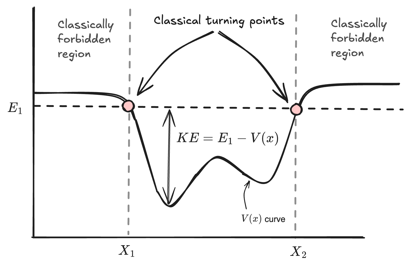 Some notes on vocabulary:
-
Classically-forbidden region: kinetic energy can't be negative. Since , any region where is called classically forbidden, since it would imply a negative kinetic energy. The edges of the well by each side are called classical turning points.
-
Classical turning points: locations where . The particle has only potential energy (no kinetic), and must "turn around" to go back into the well.
-
Particles within the well are in bound states, while those outside the well are in unbound states.
The extent of the allowed and forbidden regions depends on our total energy used for a particular bound state. might be less than , and might change from particle to particle.
Infinite Square Well
The classical model for a particle well is a ball bouncing between two perfectly elastic walls, like the old bouncing DVD screensaver. A simple model for a bound particle follows the same rules:
- The ball flies freely between the walls
- The ball is reflected perfectly at each bounce
- The ball remains in the box regardless how fast it is

Let's find the energy eigenstates & eigenvalues using the energy eigenvalue equation. Outside the box, , so which is satisfied only if (a nice thought) or if everywhere outside the box. Inside the box, , so We already know , and is confined to a box of size . We need to find our total energy and the wave function . Rewriting our EEQ,
Above, and is defined as the wave vector.
The solution to this equation is There are three unknowns: , and , which contains our total energy . We can find two of them with our boundary conditions: and . At , so . At with , which is zero if (implying a full-zero wave function, not very useful, or when for , allowing us to define yet another quantity :
is called the quantum number, while is the quantization condition.

If we use this quantization condition as the wave vector , then we can solve for our total energy as
with allowed energy eigenstate wave functions
Our final constant can be solved for by normalizing the wave function to unity, such that
leading us to the final definition of our wave equation,
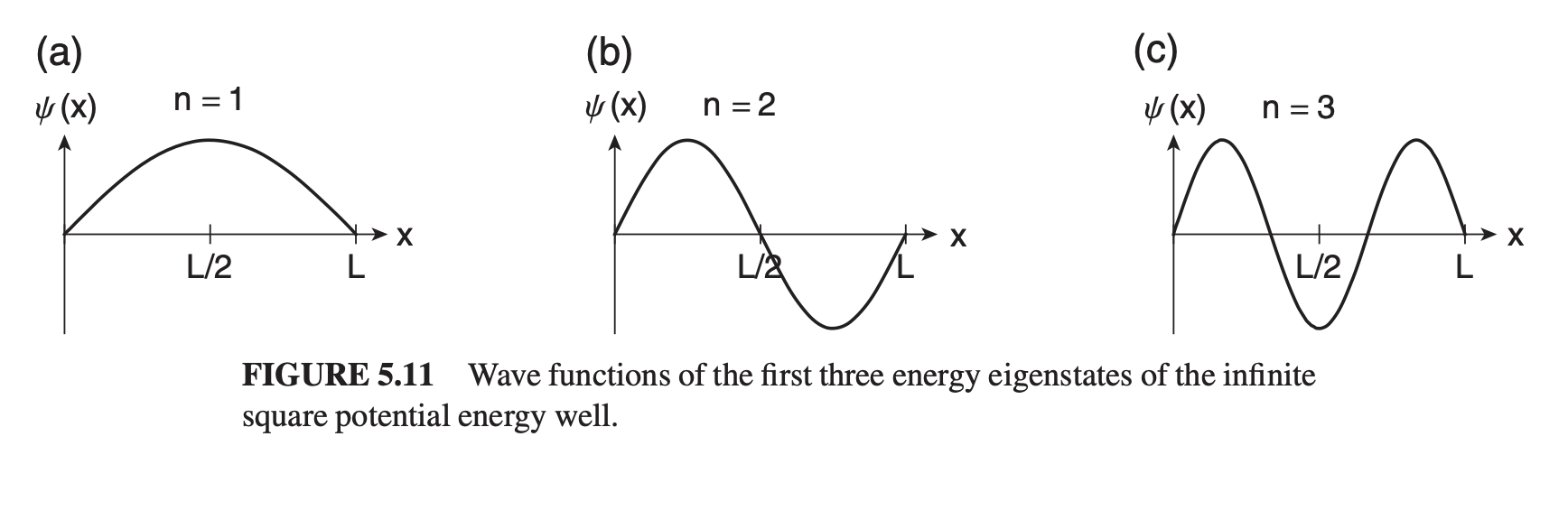 Since probability density can be calculated from some wave equation (which represents probability amplitude) via , then our quantized probability density becomes
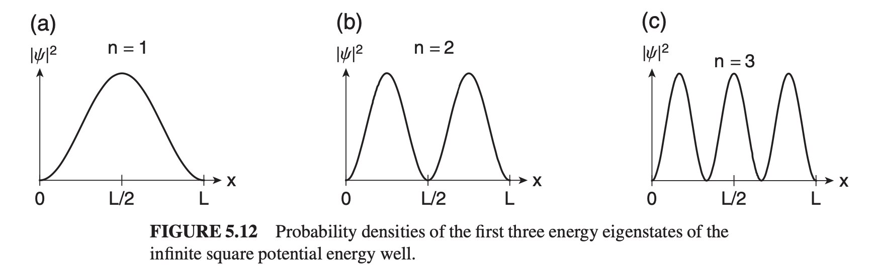 We can visualize these wave functions for different quantum numbers (and hence energy levels) like this:

Finite Square Well
 Now, our energy eigenvalue equation outside the well becomes
while inside the well it remains
When we were forced to always have our particle sitting in the well, we only needed to worry about our wave number - let's also now set up to represent the case when the particle is outside the well.
For bound states (i.e. when both inside and outside the well), and are real, so our EEVs are
with general solutions
where the even, odd values are applied to the energy levels (i.e. are odd).
Now, our energy eigenvalue equation outside the well becomes
while inside the well it remains
When we were forced to always have our particle sitting in the well, we only needed to worry about our wave number - let's also now set up to represent the case when the particle is outside the well.
For bound states (i.e. when both inside and outside the well), and are real, so our EEVs are
with general solutions
where the even, odd values are applied to the energy levels (i.e. are odd).
Let's start with the even constants. At each boundary and , the solutions are the same since we positioned our "zero point" between them. with the normalization constant providing the third equation for all three unknowns (, , ). Dividing the two above equations gives which is equivalently (by substituting in our and formulae) Similarly for the odd solutions:
We can simplify all of this by creating some new constants , and , such that so
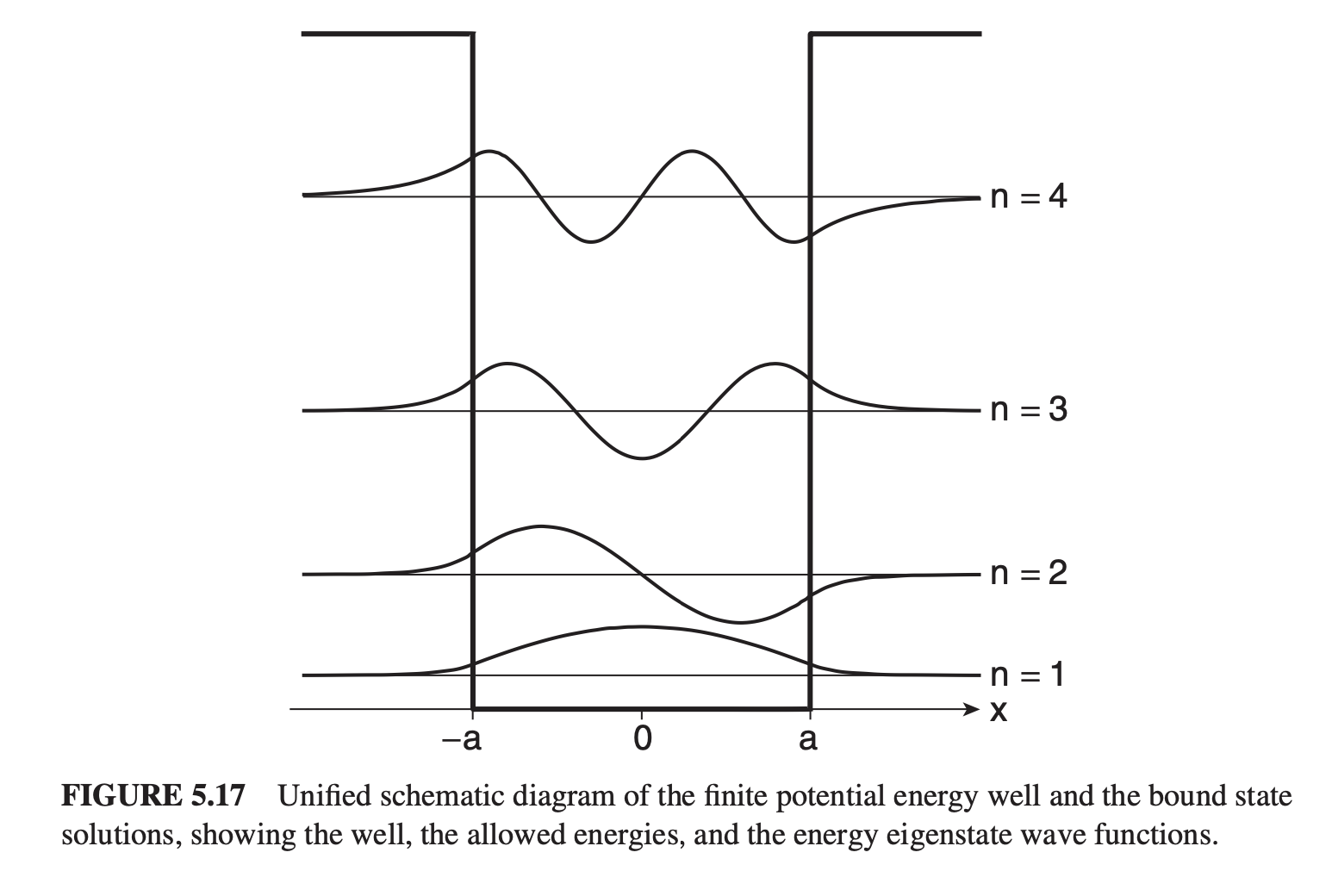
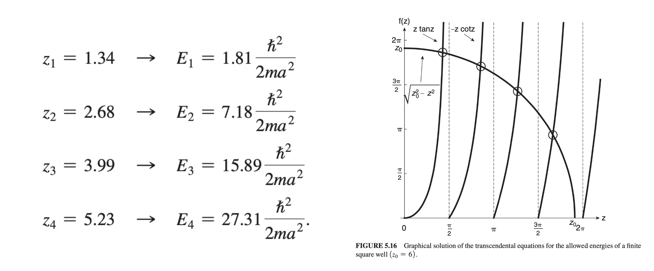
Chapter 6 - Unbound States
Reference Quantum Mechanics: A Paradigms Approach by David McIntyre.
In bound states, the energy levels of particles are quantized - they are restricted to specific values. In unbound states, energy is no longer quantized, and operates on a continuum.
We still, however, will use the energy eigenvalue equation, its associated Hamiltonian, and the energy eigenvalue wave differential equation.
Free particle eigenstates
For a free particle, is zero everywhere, so the EEV differential equation becomes where . This has the general solution of Since we're no longer in a bound state, we no longer have constraints on extrema (except for the normalization condition) - and hence continuous energy, no longer quantized. We can apply the Schrödinger time evolution to this by multiplying the energy basis (above) by a phase factor, such that Using the Planck energy relation , This wave function represents a wave that retains its shape as it moves, with a speed determined by , the phase velocity.
Thus, represents the part moving in the positive direction, while represents the part moving in the negative direction.
We can also use to represent the wave vector eigenstates, with the sign of indicating the direction of motion.
Note: we need both positive and negative values to make a general energy eigenstate.
Momentum Eigenstates & de Broglie Relation
The momentum eigenvalue equation is
This is equivalently in braket notation.
Applying to above, implying that is the momentum eigenvalue with an associated eigenstate
Note: this is a function of position , not momentum : is the independent variable while is the particular momentum eigenvalue.
Since , we can use our momentum eigenvalue to create the de Broglie relation: The momentum eigenstates are also energy eigenstates for our free particle, with energy
This means that the momentum and energy operators commute. Any given momentum eigenstate will have some energy given by the above equation, but some energy state doesn't necessarily have a definite momentum, since a single energy state usually corresponds to 2+ momentum states - meaning the energy state is degenerate.
Momentum W.E.
The time-dependent wave equation governing a momentum eigenstate is
with a probability density given by
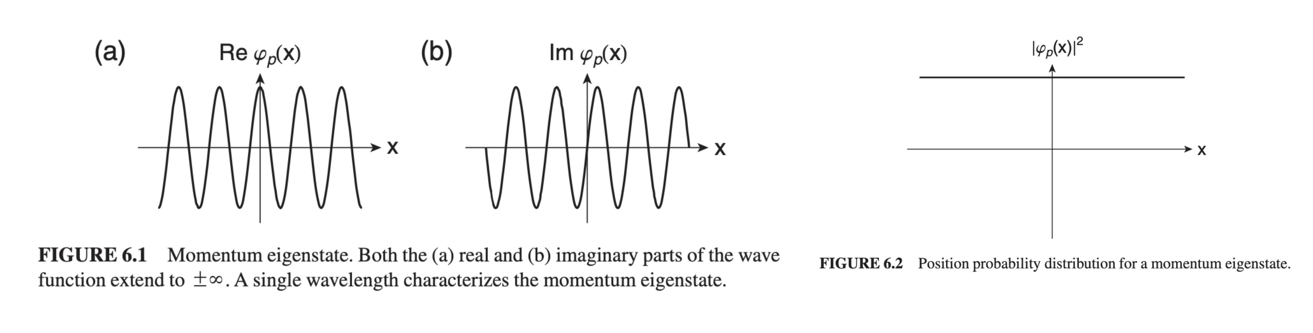 Unfortunately, this momentum eigenstate is constant regardless of position - it is spread out over all space unto . This makes the momentum eigenstate impossible to normalize - unless we create a superposition of momentum eigenstates to create wave packets.
Review on Basis States:
All basis state should demonstrate
with the orthogonality and normalization conditions able to be written in the form of the Kronecker delta: The Dirac delta function is the Kronecker delta used for continuous, rather than discrete sets, where is a function that is zero for all , except at , where it is infinite.
Thus, the orthonormality condition for the momentum eigenstate can be expressed in Dirac notation like this: which can be translated into wave function notation using the rules from Chapter 5: If we define our normalization constant then our normalized momentum eigenstates are
Momentum P.D.
If we wanted to find the probability amplitude for some general state to have momentum (i.e the projection of the general state onto momentum basis ), we'd want to find ... however, we're using in place of in our wave-function.

... but wait! and are not the same functions. They're the general state operating in different bases.
So ... let's just represent this momentum wave function with a different symbol instead. This is known as the momentum space wave function, a continuous wave function that represents the quantum state vector in terms of the momentum eigenstates.
The sinusoidal waves that make up this momentum eigenstate can be combined using the Fourier transform of to form a combined "wave packet" with a location in the basis, given by ... which we can also write in the basis with an inverse Fourier transform:
Wave Packets
Wave packets are localized superpositions of smaller waves that obey constructive and destructive interference.
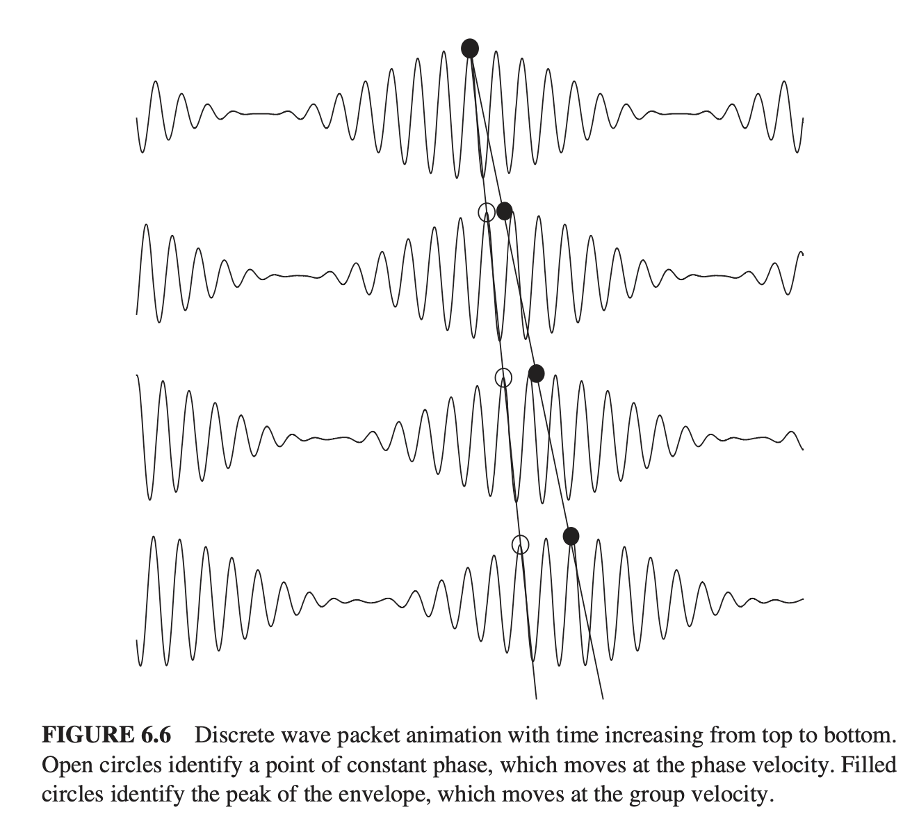
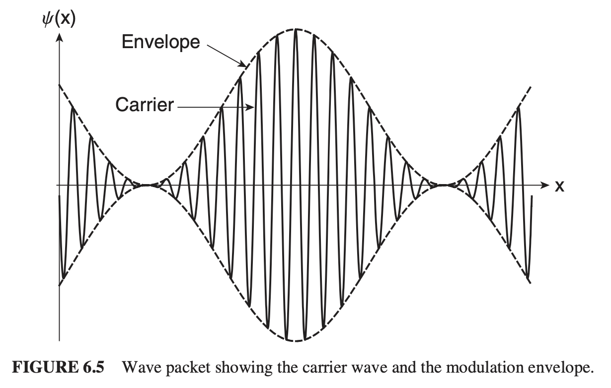 The wave packet envelope and carrier often move at different speeds. There is much more to this chapter, but I think I'll call it here for now and write up a study guide for the imminent final.
Chapter 16 - Quantum Computing
In the 1980s, Feynman asked "Can a classical computer reliably model a quantum mechanical system?" - initially, the answer was no, since the Hilbert space scales based on the number of particles involved by a factor of ...
... except ... nature does this anyway, regardless of the complexity involved.
Thus, enter the quantum computer - at least, the idea of it.
Qubits - Quantum Bits
Classical computing uses binary digits (bits) to store information: 0 or 1. These numbers are strung together to represent larger numbers (1000101), but fundamentally use transistors that are either on or off (binary states).
In quantum information systems, information is stored in quantum bits (qubits) - each a two-state system: The key difference is that qubits can exist in superposition states - where the state of the processor isn't only 0/1, but rather with probabilities of measuring each state as or , as opposed to classically 100% either 0 or 1. As we include more qubits, we exponentially increase the information storage capacity of the system: and the general superposition state is For an -qubit system, a single superposition state contains coefficients to represent information - compared to a classical system, where though bits has possible states, each state contains only bits of information.
However - if we measure a state, the system state vector collapses from superposition onto the measured state vector - so we can only extract pieces of information from our system. We can get around this with quantum parallelism, as a consequence of quantum entanglement.
Entangled States
The EPR state is entangled because measurements on one spin are perfectly anti-correlated with measurements on the other spin. It's the fourth of a set of Bell states, the complete set being This set is known as the Bell basis. Measuring one qubit in an entangled state affects the other (regardless of its location) instantaneously, allowing us to achieve the aforementioned parallel measurements - as long as we're clever about data organization.
We can also have 2-qubit product states which are expressed as a product of 1-qubit states
Quantum algorithms are not immune to the probabilistic nature of quantum mechanics - if the same program is run twice on a quantum computer the result may not be the same twice over. However, it allows us to produce answers in many, many fewer steps than a classical computer.
This is why the idea of a binary-quantum processor is popular - both have strengths and weaknesses that each "half" makes up for.
About CLAS 420
Course: CLAS 420 - Freedom in Ancient Rome and the Modern World
Professor: Dr. Joseph Bringman
Dates: Sp. 2025
Texts:
- Volume 1: Freedom in the Making of Western Culture
- By Orlando Patterson (required)
- Basic Books 1992
- Cicero. The Republic and the Laws
- Rudd, N., trans./Powell, J. edit. (2009)
- Oxford World Classics
Additional readings of Plato, Cicero, Livy, Horace, Seneca the Younger, Tacitus, Pliny the Younger, Epictetus, Appian, Marcus Aurelius, Cassius Dio, St. Augustine, etc.
Lecture 1
Concepts and conceptions
- Concepts: universal, abstract idea that captures some 'essential meaning' of something.
- Universal: applies to all instances of a type.
- Abstract: no concrete particularities (time, place, context).
- Essential: core, unchanging feature of a thing that makes it what it is.
- Conception: specific articulation or interpretation of a concept - almost like 'applied concepts'. Context, circumstance, intent is applied to a concept.
i.e. Justice (see Theory of Justice by John Rawls): all men have a conception of justice - however, many of these conceptions disagree with one another. Thus, the concept of justice is distinct from the various conceptions of justice.
Freedom
- Is it universal (single timeless meaning)? Does it depend on context?
- Is it positive ("freedom to")? Or negative ("freedom from")?
- Individual, collectives, or both?
- Is it a feeling? Quality? State of being? Measurable condition? Tied to accountability or independent of obligations to others?
- Where does it come from? Innate right?
- What is its opposition?
- Why does it matter?
- Is it fundamentally good?
We have numerous conceptions of freedom: Stoicism's 'freedom of the mind', Christianity's freedom from sin and death, Hobbesian social contract (naturally free but surrenders some freedom to government for self-preservation). Lockean liberalism (life, liberty, property), Kantian autonomy (self-legislation).
Re: Orlando Patterson and his Freedom
- Jamaican-American sociologist whose scholarship focuses on slavery and race in the Americas.
- Published Slavery and Social Death in 1982 (slaves are a 'type of death' (social death)).
- 1991 - published "Freedom: Volume I: Freedom In The Making Of Western Culture".
- Examines freedom in opposition to slavery, argues that slavery is crucial in generating the valuation of freedom as an ideal uniquely in Western civilization.
- Q: Freedom exists as a dichotomy with slavery? I.e. slavery conceptualizes freedom?
Has four questions in the intro:
- How and why was freedom initially constructed as a social value?
- How and why did it emerge as the premiere and supreme value distinct from any other potentially equally important values?
- Why did this rise to culturally supremacy happen only in the Western world, and why for so many centuries remain confined to Western civilization?
- Having achieved preeminence, what forces maintained its status as the core value of Western civilization?
Note: Patterson defines 'Western world' as Greece, Rome, western Europe.
Analyzes freedom as a sociologist and historian, seeking to understand how freedom was conceived of (and valued by) people in historical societies. Not a philosopher in this context - doesn't seek a 'true definition' of freedom.
Patterson's Conception of Freedom
Calls it a "chordal triad".
- Personal freedom: autonomy to act as one pleases, free from undue restraint, conditioned by respect for others' rights.
- Sovereignal freedom: power to act as one pleases, regardless of the wishes of others. (Associated with those who have power over other individuals).
- Civic freedom: capacity of adult members of some community to participate within that community and make meaningful decisions regarding its operation.
Dr. Joseph Bringman: What Freedom Is
Somewhat self-deprecatingly, Dr. Bringman hence declares the below to be the definition of freedom:
Freedom: "the rational capacity of a being to direct itself toward its proper good through deliberate choice."
- Rational capacity: freedom requires reason, distinguishing it from instinct or necessity.
- Self-direction: active power of self-motivation, rooted in the will.
- Proper good: aims at a certain end (e.g. flourishing - called eudaimonia by Aristotle).
- Deliberate choice: freedom is an intentional decision.
Other "sub"-conceptions of freedom:
Volitional conception: "the rational capacity of the soul to direct itself toward the universal good through deliberate choice."
- Proper good is the person's ultimate end, and the focus is internal - the will's power to choose among 'Goods' presented by the intellect.
- Often called 'freedom of will' or 'free will'.
Social freedom: "the rational capacity of a person to direct themself toward the common good through deliberate choice within a community."
- Proper good is the flourishing of society (i.e. justice, peace) and the conflict is external.
- Presupplies free will, applies it to a life in human society.
- Not just a legal status - the capacity of a person to participate in society.
- "Slave" vs "free person".
- This is a spectrum.
Political freedom / Moral freedom
Spiritual freedom: "the rational capacity of a person, perfected by divine grace, to direct themself toward union with God through deliberate choice."
- Proper good is divine communion.
- Grace elevates the will's natural capacity to overcome the distortions of sin.
- Fullest expression of freedom.
Lecture 2
Plato (c. 428-348 BC)
- Student of Socrates, whom he made a character in philosophical dialogues.
Patterson claimed Rome did not produce any original philosophers of the calibre of Socrates or Plato - is this truly the case?

- Plato was anti-materialistic, anti-mechanistic, anti-normalist, anti-relativist (was an absolutist).
- Prior to Plato was the Sophists - teaching how to conduct eloquent speech with little content.
- Anti-skeptic.
Theory of Ideas / Forms
- Postulated two worlds: visible (changing, mutable) and intelligible (eternally unchanging).
- Intelligible is unreachable physically, but we interact with it with ideas of things (i.e. intelligible is the concept).
- Visible is the form, which is the instanced versions of the intelligible.
I.e. Plato's cave:
- Shadows on the wall are the Visible World.
- The cave outside the cave = the Ideas (true reality).
- Persons within the cave = non-philosophers.
Plato and Freedom
- Plato grapples philosophically with freedom
- In 375 BC, wrote Republic
- Attempts to define the idea & form of justice, leading to other high-level stuff and things and thusly attempts to reach some 'ideal state in which justice is promoted' sort of like an absolute vacuum for photons to scoot through.
- Plato proposes three classes: drones, guardians, governing class (philosopher king).
Plato's five regimes:
- Aristocracy (rule by the best): ruled by philosopher-kings who display wisdom and seek the common good.
- Timocracy (rule by honor): rulers are ambitious and honor-focused, pursuing glory rather than wisdom.
- Oligarchy (rule by the few): wealthy few rule, valuing money over virtue.
- Democracy (rule by the people): all desires given equal weight.
- Tyranny (rule by a tyrant): single ruler seizes power and presents own desires as overriding to all others.
This is a subsequence, like a decaying element - aristocracy inevitably decays into a timocracy, which decays into an oligarchy, then democracy, then into tyranny.
Worrisome, in the right now.
Plato worries democracy would inevitably lead to every individual trying to get more than their fair share - until one single individual with 'sovereignal freedom' uses the democracy's institutions against its citizens.
- Thought aristocracy was the best government, but internal flaws (improper education of the youth) would inevitably lead to deterioration into a timocracy (honor over reason).
- Plato cites two fundamental key issues with different government:
- Money (and unstable accumulations of it, like trash heaps) (lead to individuals respecting money more than virtue)
- Factionalism
- Proposed human soul has three main parts: reason, spiritedness, appetites.
- Aristocracy keeps all three in harmony
- Timocracy emphasizes spiritedness
- Oligarchy appetites
- Democracy is a chaotic free-for-all where all three desires are given free reign
- Tyranny - individual is slave to appetites, own reason, own spiritedness, otherwise unmoored from regulatory counsel.
Q: Do you, Dr. Bringman, have any opinions on this? Recent events, Red Rising & your class have me considering the virtues of other political systems.
Frustration with difference between eloquent appetites/spirit and perhaps ineloquent reasoning, and it's
Tyranny vs aristocracy requires (most) participants believe in the same fundamental concept of absolute good? Platonic society.
Computer thing?
Lecture 3
Titus Livius (Livy) wrote History of Rome in 142 books, 35 of which still survive to today, which sought to detail Rome's history from it's founding in 753 BC to the death of Drusus in 9 BC.
753: Founded by Romulus and Remus. 509: Tarquin overthrown; Republic established. 264-241: First Punic War 218-201: Second Punic War 149-146: Third Punic War, Carthage destroyed. 133: Tiberius Gracchus assassinated 54: De Republica (The Republic) 44: Caesar assasinated 31: Octavian defeats Antony to become Rome's sole ruler 27: Octavian renamed Augustus, Rome becomes a monarchy (though Romans don't call it as such, the Greeks are honest about it).
Cicero and Plato's Republic
- Plato was high-level and abstract in Republic
- Plato was also the high-level Greek author the Romans tended to learn from.
- Romans would call the Greeks great, except for at Politics, within which the Romans outdid them.
- Cicero likely would have disagreed about Plato's ideas on freedom.
Regarding Cicero
106 BC: born in Arpinum on Jan. 3 63 BC: Becomes a Roman Consul. Quashes Cataline's Conspiracy, making him rather popular within the ruling class. 58 BC: exiled by the tribune Clodius Pulcher 57 BC: Recalled at the behest of Pompey (general, statesman) at the behest of Milo (political agitator). 51-50 BC: made governor of Cilicia, sacked 'some stronghold of rebels' called Pindenissum. 49 BC: half-heartedly sided with the Pompeians during the Roman Civil War. 47 BC: Cicero returns to Rome and receives pardon from Caesar 44-43 BC: delivered 14 Philippics (oratics/denouncements) against the consul Mark Antony. 43 BC: proscribed by the Triumvirate and beheaded.
Education
- Student of Philo of Larissa, the Academy of Plato's final scholarch. Came to Rome in 87 BC.
- Principally an Academic Skeptic, but in adherence to that was not dogmatic about it, 'heard out' other schools of thought.
De Re Publica
Republic = libertas (not ruled by kings)
- De Re Publica is first installment of his own political philosophy works.
- Acted as a justification of the Roman Republic by writing a Roman version of Plato's republic.
- Conceptualization of the Platonic ideal of Rome.
- Mostly lost to time, only fragments survive.
- Book 2: Scipio points out that Rome was a very long time in the making.
- Constitution (political system) in Latin is res publica. Denotes things that collectively concern political life.
Enter: ze Kings
- Numa (2nd king): introduces serious religion in Rome.
- Cicero: religion and humane behavior allow state to survive
- Cicero notes Greek influences are positive wrt Roman education
- Ancus Marcus - state leapt forward in culture when Greek philosophy and art are combined with Roman politics and warfare.
- Lucius Tarquinius: First Etruscan king.
- Things start going bad.
- Servius Tullius (servus means slave?), adopted son of Tarquinius I.
- Reformed Roman politics, reorganizing population, distributing them into new groups so wealthy could hold power. Democracy is dangerous.
- Servius' system is the foundation upon which the upcoming Republic was built.
- Cicero: monarchy is the enemy of freedom. A just tyrant is still a tyrant.
- Tarquin the Proud/Arrogant: kills Servius, becomes tyrant.
- Tarquin (son-in-law) and Tullia (younger daughter of Servius)
- Cicero: a successful state needs a little freedom but not too much. A good statesman should be practical.
Regarding Livy
- Augustan-era writer (Octavian renamed to Augustus) who lived during times of extreme political change in Rome.
- "What happens to a society that abandons its moral compass?"
- Livy names Augustus three times, seeming to like him but implying criticisms certain acts of his.
- Book 1: monarchy period is a collection of 'fables'.
- Implied Servius might have ended the monarchy
- Tends to be rather dramatic, likes to imagine history as almost a Greek tragedy.
509 BC: monarchy ostensibly ends. Livy's books tend to become more historical than dramatic from this point.
Overthrow of the Monarchy
- Tarquin made large unpopular public works projects, forcing Roman citizens to labor at these.
- Sextus Tarquinius (son of Tarquin) violates Lucretia (Collatinius' wife). She summons her father, husband and tells them of it, then commits suicide.
- Sextus is awful.
- Monarchy is summarily overthrown afterward.
- Revolution led by Lucius Junius Brutus (Brutis = stupid, cultivated name but obviously not accurate), king replaced by consuls.
- Consul's oath of office says they wouldn't be a king, Livy's Brutus' speech includes language used in the oath.
- Brutus: hero insofar as he removed a tyrant. Would have been wicked/bad to remove Servius.
- Cicero: Roman Republic was only successful because it developed over a long period of time.
Lecture 4
When the Roman Republic was first formed (~509 BC) after the overthrow of Tarquinius the Arrogant (Superbus), it was predominantly governed by patricians - effectively aristocrats.
Over time, the working-class plebians (regular citizens) demanded more rights from the patricians. This wasn't done easily - but primarily through general strikes known as the Conflict of the Orders.
1. 494 BC, established tribunes of the plebs
- Many plebians experiencing financial hardship and indebted to patricians
- Consul Appius Claudius I decreed debtors may be imprisoned by creditors
- Plebians organize, depart Rome to neighboring Sacred Mount
- Patricians can't staff armies, nobody really in Rome.
- Patricians form tribune of the plebeians from plebeians
- Meant to safeguard plebeians from patrician abuses
- Plebeians collectively swear to kill anyone who harms a tribune, making them sacrosanct (despite not having a ton of power)
- Tribunes can stop patrician magistrates by just physically standing in their way
The tribunician power was initially only negative (veto rather than enact laws themselves), citizens also have the right to appeal to the people in the event of a magistrate sentencing someone to death or greivous punishment.
2. 449 BC, ended Decemvirate
In the early republic, Roman law was initially strictly oral, passed down by the patricians. Athens did the same (before Draco).
- In 450, laws written down in the Twelve Tables. Ten patricians selected and given total authority while in office.
- Only wrote ten tables initially.
- These patricians were called the Decemviri (or Decemvirate).
- All magistraceries (and tribunate) suspended, as well as the right to appeal the decemvirate's decisions (suspended)
- Surprisingly, the first ten wrote their tables, stepped down and all was alright.
In 449, a new decemvirate was elected to write two more tables.
- Appius Claudius II was said (by Livy) to have rigged the election in favor of himself and his cronies.
- Killed, imprisoned and fined without trial anyone who opposed them, permitting no appeals.
- After the one-year office term ended, didn't hold new elections and killed anyone who disagreed with their rule.
Enter: Verginia, daughter of Lucius Verginius, centurion in the Roman army. Appius Claudius was romantically interested in her, but V. rejected his advances, so he declared her his slave and required her return to him.
Claudius declares Verginius was the only one able to legally defend her, but was away with the army. Claudius attempted to prevent Verginius's return, but Verginius regardless manages to return. Claudius declares himself the judge of this case, refused to hear out Verginius, and demands Verginia to be delivered to him regardless.
Verginius kills his daughter to prevent her becoming a slave, declaring to Claudius "By this blood, Appius, I devote thy head to the infernal gods".
Note: this is all according to Livy, who is quite a dramatist.
Plebeians go on strike once more after hearing what happened. Senate eventually gives into them, decemvirate is abolished, tribunes restored and appeals guaranteed as the right of citizens.
3. 445 BC, repealed intermarriage prohibition
Nothing significantly notable here except for the consequence.
4. 342 BC (obscure military revolt?)
5. 287 BC, gave plebians full equality and ability to enact their own laws
- No approval required by the patricians or senate.
- By the time of the late Roman Republic and early Empire, patricians were a 'token class'.
Note: Patrician-Plebeian divide generally ends at this point, now divides are mostly based on wealth alone.
Lecture 5
Digest of Justinian:
- Condensation / clarification of juristic writings, compiled in the 530s AD
- Freedom is natural / slavery is unnatural
- Is freedom a natural right? Is it only able to be removed via unnatural (i.e. civilized) methods?
In 287 BC, the lex Hortensia was passed after the 5th secession of the plebs, making the resolutions of the Plebian Assembly binding laws. - Every citizen is now able to contribute to the passage of laws
Regarding Libertas
Is liberty natural?
Wirszubski p.7: true libertas is not the right to do whatever you wish.
- Such unconstrained conduct would be licentia, or irresponsible freedom, not libertas.
- See Chapter 1 - General Characteristics of Libertas:
There is profound truth in Cicero's saying, “legum idcirco omnes servi sumus ut liberi esse possimus”. For were it not for the restrictions imposed by law, everyone would be free to do always as he liked, and that would result—to use Hobbes' phrase—in a “bellum omnium contra omnes”, that is to say, it would result, not in the enjoyment of complete freedom, but in its self-destruction through excess. Fools, observed Tacitus, identified licentia with libertas.
- Prerequisite for libertas is the renouncement of self-willed actions
- Libertas enjoyable only under the law: without law, no freedom
- Cicero: "we are all slaves to the law that we may be free"
Personal note: I sense this idea of freedom, libertas, as freedom with an attached responsibility, is not one to be dismissed lightly. Cicero holds it in contrast to licentia - or a freedom without responsibility, 'deserted island freedom'.
- libertas is consistent with the disciplinia Romana - the right of a citizen in an organized state.
- Not freedom of individuals, but rather a citizen's place in the community - agency within this civic community, but roles should be responsibly performed to maintain a stable state.
- Not autonomy of will, but rather social relationship with both rights and duties.
- Rights in libertas must be equal for all - libertas is the upper limits of political freedom.
Political office in the Republic
Note: the Romans were, at no point, egalitarians: believed in hierarchies in society (wealth, birth, etc). Hierarchy was an accepted notion.
- Aequae libertas: equality before the law, same laws applicable to everyone, but not equal political rights for all.
- Same legal standards, not necessarily political/social standards
- I.e. property requirement for political office was generally acceptable.
- Political jobs are full-time careers
- But no salaries - politicians needed to be independently wealthy
Roman politics was very dissimilar to Athenian democracy in this respect, which was decided by lot rather than wealth. Required both wealth and land.
Personal note: Rome had some, but not a lot, of political historical precedent to reference - the negative connotations associated with oligarchies (and democracies) today were not (necessarily) widespread concerns then.
- It was preferred for political office-holders to have familial precedent within politics - my great-grandfather was so-and-so, I have his blood, therefore ...
Wars of conquest
Series of major events between 287 and 133.
- By 287, Rome controls all of Italy, and begins expanding outward.
- 261-242: First Punic War
- 218-201: Second Punic War, Rome becomes established as the most powerful country in the Mediterranean (note: Carthage remains active during this time, but defeated in two separate wars by Rome now).
- 214-148: Rome invited to intervene in various conflicts between Greek kingdoms; eventually the Greek islands are fully annexed into Rome.
- Note: 336-323 BC, Alexander the Great of Macedon conquered much of the known world after unifying Greece. Greece fell apart after his death.
- Note 2: Aristotle tutored Alexander the Great - 287 in Rome was just ~fifty years after Aristotle's death (322 BC).
- 146: Rome concludes the Third Punic War by destroying Carthage.
Gracci period ~133 BC
Following these conquests, Romans have a ridiculous amount of land and even more slaves.
- This influx of land was predominantly given to the rich.
- In 133, Tiberius and Gaius Gracchus (Gracci brothers) active.
Most of our knowledge of this time is covered by Appian of Alexandria c. 141 AD, wrote the Roman History (24 books), generally held to be a good source re: the Gracci period and following. Pays close attention to the plight of the working class.
In the decades preceding 133, many Roman small farms fell into disrepair as owners were sent off to war in far-off lands.
- Roman army still mostly composed of conscripts rather than professional soldiers.
- Many wealthy neighbors bought up (or stole) nearby farms while owners on campaign; when they returned, many vets found themselves displaced.
- Or indebted to large landowners
- Large landowners also started to amass large supplies of slaves to provide cheap labor on their vast estates (latifundia = slave-worked large farm)
- Incredibly large wealth discrepancies arose during this point.
Civil War (Appian)
Referenced PDF on Appian's Civil War.
- Many cases of leaders who just wouldn't give up power; factionalism.
- Rome confiscated Italian lands, set out colonies
- Rich got possession of undistributed land
- Tiberius Gracchus, tribune of the plebs, wanted new law to redistribute land (Gracchus land reform).
- Proposed limiting land holdings to 250 jugera (~150 acres).
- Marcus Octavius vetoes this (fellow tribune)
Tiberius Gracchus - Revolution by Legislation
- Elected tribune of the plebs in 133 BC
- Knows land reform is very popular with the masses
- To overcome opposition to agrarian reform law, deposes Marcus Octavius - an unprecedented (and arguably illegal) action
- Ti. Gracchus: tribunes should be recallable if they do not act in the people's interests - revolutionary proposition.
- Appian: Tiberius gathered a bodyguard to himself with the intention of forcing Octavius to comply, even if he doesn't want to.
- Plebian assembly votes to remove Octavius and enacts the land reform law.
This land reform law (and the actions taken to enact it) is regarded as the spark that set the Republic ablaze.
- Tiberius seeks reelection to tribune as his term comes to a close, since he knows he'll be in a lot of danger after his term ends.
- Unfortunately, most supporters from countryside - leave back to countryside after vote held (Appian 1.13.57)
- T. Gracchus's foes (of which there are many at this point) accuse T. of aspiring to kingship and seek to disrupt his reelection.
- Violence breaks out between both sides (Plutarch: Tiberius's enemies started it. Appian: blames Tiberius for inciting supporters to violence).
Then: Cornelius Scipio (pontifex maximus, head of state religion, 'supreme pontiff') rushes at Gracchans (who of course let him in due to position), followed by senators.
- Scipio is quite conservative, not happy with land reforms.
- Kills Tiberius Gracchus (133 BC) - first open political assassination in a very long time, as well as many of his supporters.
Sic mors
Appian: killing was an abominable crime, the first to be committed in the public assembly, and led to a lot of similar events soon after.
Vell. Pat. 2.3.3: beginning of civil bloodshed and assassination without fear of punishment in Rome. From now, right overwhelmed by right, power took precedence. Differences between citizens were remedied by sword rather than word, wars started not for cause but on the basis of their profitability.
- Doesn't truly take effect until the death of Gaius Gracchus.
Enter: Gaius Gracchus
Roughly a decade after Ti. Gracchus's death (~123 BC), younger brother Gaius Gracchus elected tribune of the plebs.
- Gaius not only champions Ti. Gracchus's land reform but extends his political agenda to questions of citizenship - wanted to grant Italians citizenship.
- Tiberius: interested in land distribution. Gaius: interested in effectively remaking Roman politics on a far grander scale.
- Instituted a lot of reforms, including stripping senators of the ability to control juries, instituted a grain dole, etc.
- https://en.wikipedia.org/wiki/Cura_annonae - gave out subsidized bread and grain for free to many citizens.
- Instituted a lot of reforms, including stripping senators of the ability to control juries, instituted a grain dole, etc.
Note: rather than speaking to the Roman senate / aristocracy, Gaius spoke in assemblies toward the masses / people.
- Runs for reelection to the tribune, second term. Loses when he runs for a third term however.
- Violence breaks out in the voting place, citizen killed by his followers, whose death is blamed on Gaius
- Retires with followers to the Aventine Hill (Sacred Hill), 'last stand'.
- Gaius ends up dead, second act of political killing in a decade.
- Political opponents used political unrest as an excuse to declare martial law and march on his supporters.
- Political allies purged in a series of trials (reportedly extensive purge on the order of thousands), though legislation remains mostly untouched.
Note: Gracchus brothers both sought broad political reform and both died; both deaths seem to cause widescale political unrest.
- Gracchi brothers became symbols of resistance to oppressive, greedy landowners
- Political violence unleashed in their era would later spiral out of control, setting in the process whereby the Republic would unravel and later perish.
- Appius p.19: Realization that the tribunate had been debased/weaponized as a tool of the powerful set in (such as by Marcus Octavius).
- Started off as a means to defend against aristocratic oppression - later gave way to tribunes accepting bribes from wealthy aristocrats.
- After Gracchi, populares vs optimates.
Lecture 6 - Optimates vs. Populares
Regarding lecture 5 - the Gracchus brothers are a prime example of morally debatable figures in history. Both, in the context of the people of Rome, were platonic Good - they fought for the little things for the people. However, they also are regarded as the catalyst which led to the fall of the Republic. In this sociopolitical standpoint, they later led to a lot of misery.
Optimates: "best ones". From Wikipedia: 'Among other things, optimates have been seen as supporters of the continued authority of the senate, politicians who operated mostly in the senate, or opponents of the populares.'
Populares: "supporters of the people". From Wikipedia: 'The populares have also been seen as focusing on operating before the popular assemblies, generally in opposition to the senate, using "the populace, rather than the senate, as a means [for advantage].'
Not patrician vs. plebian, but rather based on outlook and procedural proclivities (senate vs. popular assemblies).
Politicians could on a case-by-case basis adopt "optimate" or "popularis" positions - 'politically fluid'.
I got a bit distracted here looking at Mountain Project.
Social War (91-87 BC)
- Romans kept resisting Italian demands for Roman citizenship
- So, Italians formed a league and created an uprising in 91
- Sought to create 'independent Italy'?
- Some communities remained loyal to Rome, Romans rewarded them with citizenship
- Rebelled to get citizenship - loyal ones got citizenship - lol.
- This drained support for the rebellion gradually
- Wikipedia: "The massive expansion of the citizenship that followed the Social War remained a politically-charged topic, especially in terms of how they would be allocated into voting blocks. Disputes over enfranchisement played a role in Sulla's march on Rome in 88 BC to depose plebeian tribune Publius Sulpicius Rufus."
Sulla
- Patrician aristocrat who originally served under Marius during Jugurthine War; became enemy of Marius after.
- Became consul in 88, tasked with commanding Roman army to make war against Mithradates king of Pontus.
- Pontus: very rich eastern kingdom, lots of bounty.
- Marius wants to come out of retirement to lead army; Marius's allies connive to move command from Sulla to Marius
- Tribune of the plebs gets law enacted to this end, making Marius the army's commander
- Marius sends legates to Sulla to order him to turn the army over to him.
Now.
- Sulla ends up killing Marius's legates
- Sulla appeals to the soldiers about the injustice of the proposal, calling on them to defend his honor against Marius's insulting claims to command
- All but one of Sulla's officers abandon him, but the rank-and-file troops back him, and Sulla marches on Rome.
- Marius & his allies flee Rome before Sulla took it over. Sulla becomes the first Roman general to lead his army against Rome.
- Sulla held new consular elections, which were free and fair
- One of the new consuls (Cinna) was an enemy of Sulla, so Sulla forced consuls to swear to uphold Cinna's authority regardless.
- Sulla marches off to the east and defeats Mithradates
- Marius: returns to Rome from exile, elected consul again, then persecutes Sulla's family and supporters, kills a ton of people, then dies of old age.
- "Within weeks" according to Wikipedia.
- Cinna, Marius's supporter, takes over Marius's faction and stays in office without holding elections for a number of years, until the army mutinied and kills him too.
Thus ends Marius and Cinna.
- Sulla returns to Italy in 83 BC.
- Had most of his supporters (and victorious army) with him, pretty annoyed.
- Armies defeat Marian faction, Sulla took over Rome, having himself elected dictator.
- Dictator is technically a constitutional office - useful when state is in jeopardy.
- Begins dictatorship by proscribing all his enemies (listed enemies he wanted killed for bounty).
- Reorganized government. Undoes pretty much all the stuff that gives power to the people, castrated the plebian tribune, gave Senate more authority, generally benefitted the Optimates.
- Then resigns, partied in villa for a few years until death.
- Set precedent of military force to achieve political solutions.
Julius Caesar
- Born into a blue-blooded (claims divinity) patrician family
- Formed an alliance with Pompey (old lieutenant of Sulla) and Crassus (richest man in Rome)
- Pooling resources, Caesar is elected consul in 59
Pompey, Caesar and Crassus are some of the most popular men in Rome at this point - effectively totally control Roman politics for next decade.
- 58, Caesar becomes governor of Rome's then-small Gallic province: then, conquered rest of Gaul over the next decade.
- 54, Caesar's daughter Julia (wife of Pompey) dies; Caesar and Pompey have a strained relationship after.
- 53: Crassus dies fighting the Persians
Caesar and Pompey become rivals at this point.
- 49: Pompey orchestrates to deny Caesar the right to run for reelection to consulship in absentia and orders Caesar return to Italy unarmed.
- Mark Antony (tribune of the plebs) vetoes anti-Caesar measures but is threatened by the Pompeians
- Flees to Caesar in Gaul, relates what's happened.
- Like Sulla, appeals to army.
- This time, all but a single officer rally behind him & rank and file.
- Single officer is a childhood friend of Caesar - alas.
- Crosses the Rubicon (legal boundary of Italy) and wages civil war against Pompey, emerging victorious as dictator of Rome.
Rule of Caesar
As dictator, Senate votes many honors upon Caesar.
- Starts seeming like a "dominus" to many aristocrats, who had lost their freedom since Caesar controls the govt.
Missed some stuff here - writing an email.
Brutus
Marcus Junius Brutus (descendent of legendary Brutus who overthrew Tarquin) becomes leader of the conspiracy to overthrow Caesar despite being a friend to him. Around 60-70 senators are part of the conspiracy, including Cassius (Brutus's co-leader)
15 March 44 BC, Caesar slain in the senate.
- Action was very unpopular with the Roman masses; Appian says the assassins were mistaken in thinking the people cared about 'freedom'.
- Rioting breaks out, total chaos.
- Assassins have to flee Rome.
- Mark Antony as consul claims leadership of the Caesarians and negotiates a compromise with the assassins.
- Assassins lives supposed to be spared, Caesar's actions supposed to be ratified.
Patria potestas
Patria potestas ("power of the father") relates to the power a father has over his family; it is (almost literally) a term to describe not only the patriarch but the system of patriarchy within Roman families.
I'm going to be writing a short essay on it - I'll compile my sources here and show my messy brainstorming, then attack it after.
Sources
- penelope.uchicago.edu - Bill Thayer has a comprehensive page on potestas here, as it relates to a few things, including the magisterium, the Roman family, Roman slaves. This seems to be originally defined in "A Dictionary of Greek and Roman Antiquities, John Murray, London, 1875."
- "Potestas is also one of the words by which is expressed the power that one private person has over another, the other two being Manus and Mancipium. The Potestas is either Dominica, that is, ownership as exhibited in the relation of Master and Slave [Servus]; or Patria as exhibited in the relation of Father and Child. The Mancipium was framed after the analogy of the Potestas Dominica [Mancipium]."
- It does not seem that the Patria Potestas was ever viewed among the Romans as absolutely equivalent to the Dominica Potestas, or as involving ownership of the child; and yet the original notion of the Patria came very near to that of the Dominica Potestas.
- The father could exheredate his son, he could substitute another person as heir to him [Heres], and he could by his will appoint him a tutor.
- The Patria Potestas was dissolved in various ways. [...] including by the death of the father [...] the children adopting offices (daughter: Vestal) [...] emancipation of the child by the father (?) [...] or if the father lost his citizenship.
Sidenote: I love this person's little site, his picture of him and his chicken is lovely, and I don't even know his name or anything about him other than that he has a cat named Boo and the site was made on a Macintosh 7100 (named Penelope, now retired).
- Institutes of Roman Law on DE PATRIA POTESTATE: "a man has power over his own children [...], a right peculiar to citizens of Rome, for there is scarcely any other nation where fathers are invested with such power over their children as at Rome; and this the late Emperor Hadrian declared in the edict he published respecting certain petitioners for a grant of Roman citizenship to themselves and their children [...]"
- "Patria potestas was founded on consuetudinary law" (originated from customs/practices instead of written legislature)
- "Over the person of the child the father had originally a power of life and death. [...] But in later times this power was withdrawn. Hadrian condemned to deportation a father who in the hunting-field killed his son who had committed adultery with his stepmother" [...] "Fathers retained the power of moderate chastisement, but severe punishment could only be inflicted by the magistrate"
- "Originally also parents had the power of selling (mancipandi) their children into bondage, thus producing a capitis minutio, or degradation of status"
- Only to another Roman citizen. Rule was later withdrawn, however.
Lecture 9 - Cynics
I missed a few lectures prior to this one.
Cynicism
Greek-origin philosophical system which lacked any institutional equivalent of Plato's academy, but generally concentrated on three issues:
- Nature: live in accord with human nature by realizing "people are reasoning animals", rejecting arbitrary conventions of society.
- Virtue: achieved by following one's natural sense of reason, living simply and shamelessly free from social constraints.
- Only goal of human life, only thing needed for inner happiness.
- Wealth, status, honor is pointless/irrelevant.
- Freedom: self-sufficient, reject wealth, pomp and other conventional values. Being above social conventions / unconstrained by interactions with society.
Diogenes the Cynics
One of the more famous cynics.
- Born in Sinope (412-323 BC)
- Eventually landed in Athens and became student of Antisthenes (pupil of Socrates), from whom he learned quite a lot
- Scion of a wealthy family, but embraced poverty and simplicity.
- Spurned all social conventions, great and small, not caring that he offended people.
- Some liked his eccentricity, others of course did not.
Diogenes did not like Plato (and the feeling was quite mutual).
"Looking for a man" while strolling through the agora.
Later captured by pirates, enslaved in Corinth. While there, he taught Crates of Thebes, who later taught Zeno of Citium (founder of Stoicism).
Stoicism
Stoicism was a branch of philosophy which later emerged from cynicism.
- Focused on the importance of living in accordance with nature.
- Common humanity of everyone regardless of nationality, sex or condition of servitude (slaves just as human as monarchs).
- Did not advocate abolition of slavery, but did urge humane treatment as fellow humans.
- Developed theories of natural law.
- Cicero articulated his own views on natural law which greatly influenced later thinkers (U.S. Declaration of Independence).
Virtue
- Virtue alone is good, whereas vice is the only evil.
- Both necessary and sufficient to make one happy.
- The pursuit of which is sufficient.
- Differs from other philosophical schools, such as Platonists and Aristotelians who considered virtue to be the chief, but not exclusive, good (ditto vice).
- To the Stoics: virtue is all-or-nothing. No half-assing. Either perfectly virtuous or viceful.
Virtue and vice is within one's own agency, and we have the ability to enact change within it.
However, things exist external to virtue and vice.
- Wealth, health, poverty, illness are morally indifferent / external.
- We can't affect them. Of course, wealth/heath generally positive, illness/poverty generally negative.
Stoics: virtue or vice is within one's own control whereas everything else is not, so for the Stoics good and evil is solely concerned with what is in our control / agency.
Freedom
- Stoics appreciated political freedom, put emphasis on spiritual freedom (i.e. ruling one's passions rather than vice versa = freedom from passions).
- Epictetus (50-135 CE), who was born into slavery, expounded the doctrine that slavery to one's passions was a worse evil than bodily slavery.
- Agency and ability to change.
Epictetus
c. 50-135 CE
- Greek man born into slavery in Hierapolis
- Name means "acquired"
- Ended up in Rome, sold to Epaphroitus (freedman, secretary, and suicide-assistant of Nero)
- Allowed to study philosophy under Musonius Rufus, noted Roman Stoic
- Freed sometime after Nero's death (~68 CE)
- Taught philosophy in Rome until c. 93 CE, until Emperor Domitian banished all philosophers
- Why???
- Moved to Nicopolis, where he founded a school of philosophy and taught (among others) Arrian, who wrote down teachings.
Discourse on Freedom
- Unique text on freedom from the Roman period
- One of the few writers with a surviving work who was himself also a slave at some point (first ~20 years of life)
Questions:
Who are the free and who are the slaves?
- The wicked? No - sorrows, envy, etc.
- Animals? Perhaps - but do they enjoy being cooped up?
- Servitium amoris (slavery of love) - no, bound to the person one loves
Who is a slave?
- If you are compelled to do something, you are a slave.
- To free oneself from compulsion, death.
Servile Wars
The Servile Wars were a series of three large slave revolts.
- The first two localized to Sicily (135-132, 104-100 BCE)
- Both involved slave leaders who declared themselves kings
The largest of the three, however, was led by Spartacus.
Spartacus
- Thracian man who served as a soldier alongside the Romans, before he was enslaved by aforementioned Romans.
- No eyewitness or contemporary accounts of him exist; best sources, Appian and Plutarch's Life of Crassus, written centuries after events.
- Thus, we know effectively nothing of him apart from his participation in the Third Servile War.
- Spartacus and a bunch of enslaved gladiators escaped to the countryside and sought to recover their freedom.
- What type of freedom? From slavery? Back to homeland?
- Either instigator or later chosen leader after revolt.
- Soon after escaping, band swells (slaves, fugitives, even free farmers joined up), army swelled to 100,000+ strong, moving up and down the Italian countryside.
- Managed to defeat several Roman armies.
- Romans initially dismissive of revolt, then frantically attempted to stop revolt after realizing how successful it was.
- Crassus himself got command of a Roman army, defeated Spartacus's army (with Pompey coming in near the end to 'help out')
- Spartacus and all his soldiers were crucified.
- Final major slave revolt in Roman history.
Lecture 12
I missed last lecture - this seems to start after Augustus Caesar's rule into Tiberius's rule.
Stoic opposition
Patterson (p.264) identified two strains in Roman stoicism: reactionary and reformist.
- Patrician Stoicism, a reaction to contemporary politics
- More influential under the Principate than the Republic
- Tool for survival under the Principate
- "Philosophy of consolation, life sucks under Nero"
- Seneca, Epictetus
- Reformist Stoicism, which could be a radical interpretation.
- Reforms of society at large
Manifested principally in writing and in the actions of a few individuals.
- Cato the Younger (see below)
- Brutus and Cassius were also heroized by the Stoics
- Thrasea Paetus below, opposed Nero (primary figure in stoic opposition)
Wirszubski Ch. 5
- Principate & libertas were once considered contradictory but later were mixed.
- Stoic Opposition was not attempting to restore the Republic, but rather wanted the emperor to be more like Augustus, not Nero.
- See https://en.wikipedia.org/wiki/Stoic_Opposition
- Socrates took his own life as he wouldn't admit he'd committed any crime - intellectual opposition to tyranny.
- Cato the Younger takes his own life while reading Plato's Phaedo
- Posterchild for later Stoics - model of opposition to tyranny
- https://en.wikipedia.org/wiki/Cato_the_Younger#Final_campaign_and_death
- "Caesar is said to have responded to his death by lamenting that Cato's death meant Caesar could not pardon him."
- "After righting the city's financial accounts and disbursing the remaining monies to the city's inhabitants, Cato discussed with his friends at dinner the Stoic belief that a truly free man would never become a slave."
- Wow. He seems a good man.
Libertas Senatus
- "Freedom of the Senate" became important in the imperial period (perhaps as a counterpoint to Imperial power?)
- Last institutional link to the Roman Republic, became important / representative of the better elements of the old Republic
- Roman people never (generally) rebelled against the emperors
- Opposition to 'despotism' was confined to the senatorial class
- Thrasea Paetus (important to Tacitus/Wirszubski) senator who constantly opposed Nero in dramatic ways
Exitus literature
Exitus literature: biographies of famous men that focus on their deaths ('exitus', generally by suicide), often Stoics, which were popular among the Stoic opposition.
- Several biographies of Cato the Younger were in circulation for instance
- Tacitus' Agricola is one surviving text notably influenced by this genre
- Tacitus himself never killed himself (though lived through 'bad emperor' Domitian's reign)
- Agricola was father-in-law who was governor of Britain in 77 AD by Domitian, who later persecuted him out of paranoia
- Agricola never took his own life despite imperial prosecution - Tacitus cited him as 'a great man under a bad emperor' (though Tacitus himself is of course biased).
Marcus Aurelius (161-180 AD)
Roman emperor, last of the Five Good Emperors
- Wrote Meditations, private reflections not intended for general publication.
- Written in Greek (not Latin!), though contextually appropriate as Meditations covered a lot of originally Greek philosophy.
- Reflections: who knows why he wrote them, but in my mind I wonder if they weren't written as reminders. Here are things that are important for myself to remember in the future.
- Wrote about how he had learned much from many of the Stoic Opposition figures (Dr. Bringman: interesting particularly given that he himself was an emperor, the very figures many of the Stoic Opposition folks tended to oppose).
Lecture 13 - Religion and Rome
Regarding separation of church and state:
- Romans might have viewed this very concept as absurd
- "Religion" had a very different connotation to everyday Romans - all sorts of religious phenomena existed as part of everyday life.
- How can any aspect of life escape being included in the gods' providence? ... no significant decisions in life unaffected by religion.
- (p. 128) nobody may have private gods unless brought in officially, or ancestral gods worshipped in private.
- Should be state-sanctioned gods
- Roman religion generally quite practical, not spiritual.
- Intellectuals often became very attached to mystery religions
Bacchanalia affair: more a suppression of a social phenomenon than religious repression.
Trajan: as long as suspected Christians openly worship the Roman gods, we don't care too much about their past activity.
Patterson 187-190: Free Will / Epicurianism
Epicurianism: a more wholesome version of hedonism. Pleasure is the ultimate good, but not in the sense of indulgence - pursue freedom from pain through moderation, simple living and strong friendships.
- Epicurus on free will: without free will, freedom arguments are moot.
- Take away free will, and there is no impetus to do anything at all.
- Morality is impossible without free will - how can we condemn a person whose actions are predetermined by necessity/fate?
- World without free will is sociologically impossible per Patterson.
- Epicurus: natural to be free.
- Human freedom is distinct in being chosen freedom.
Augustine
Born 354 AD in Thagaste (Souk Ahras, Algeria), about 150 miles inland from Tunis
- Berber (North African) ethnicity
- given name: Aurelius Augustinus
- Mother: Monica, a Christian
- Father: pagan
11: educated at Madaura. 17: educated in Carthage. 15 year relationship with a low-status Carthaginian woman.
- Ended relationship to become engaged to wealthy young woman ...
- Then ended that relationship to become a Christian
- Wrote Confessions
Augustine: free will is an important topic in a theological context, free will explains the existence of evil.
- Argument: why does evil exist if God is all-powerful?
- Free will given to man because man cannot do anything without it (good or evil) without it
- Given free will to use in favor of good not evil
- If man uses free will for evil, then he is responsible for his actions and is justly punished by God
Lesson 1 - Fronts, Highs, Lows
Highs and lows refer to relative pressure gradients, often showed on contour maps called synoptic charts:
 These tend to take place on the surface, as opposed to higher in the atmosphere. Historically, these were first delivered by horse, then later by telegraph - now by internet.
The light blue barbs indicate the direction wind is coming from - barb tail length indicates speed.
The solid red contours indicate regions of constant surface sea level pressure.
In the northern hemisphere, air flows:
- Clockwise (anti-cyclonic) around a high
- Counterclockwise (cyclonic) around a low
Highs are generally associated with calm weather, lows with clouds and stormy weather.
Weather fronts, introduced during WWII indicate regions of active change in pressure.
Fronts tend to be in low-pressure troughs.
Time
Meteorologists (like astronomers) use UTC (also known as GMT or Z) as a baseline time zone. or if in PDT.
In the United States, daylight savings time starts the second Sunday of March and lasts to the first Sunday in November, and transitions at local midnight.
Weather station models
Weather station models will generally take the form of this chart:
Generally, these models won't be independent entities or charts, but might be seen in surface plots (or synoptic charts) such as shown at the start of this page.
Extinction
This is how we quantify how a star's magnitude changes with the airmass between the observer and the observed star.

Unfortunately, extinction varies with wavelength, since the sky absorbs some wavelengths more intensely than others ... so we'll see different values of for each filter used.
 To correct for this, let , where is a color (i.e. ) - then,
2nd-order extinction is normally quite small (~0.04 magnitudes), but still important to include for high-precision photometry & blue stars. It can be determined with a close pair of different-color stars by fitting the slope of vs (since is a constant change-in-color for the two) - we end up with
To correct for this, let , where is a color (i.e. ) - then,
2nd-order extinction is normally quite small (~0.04 magnitudes), but still important to include for high-precision photometry & blue stars. It can be determined with a close pair of different-color stars by fitting the slope of vs (since is a constant change-in-color for the two) - we end up with
Image Reduction Pipeline
Use several Jupyter notebooks, rather than a single "The Master Notebook" - it can get long and big and slow.
- Take calibration frames (biases, flats (dome and/or sky) and darks, if necessary)
- Observe targets (science, standard stars and airmass-constraint stars (extinction stars))
- Remove instrumental signature from observations using calibration frames.
- Measure stellar fluxes (i.e. with aperture photometry or PSF photometry)
- Solve for extinction coefficients / the space magnitude
Charge-Coupled Devices (CCDs)
The CCD process:
- Light hits some detector array, triggering a tiny detector (typically 10-15 in size)
- Detector translates energy of the incident photon to some digital value
- Software confirms the receipt and reconstructs an array from the values.
High quantum efficiency (electrons per incident photon), and also generally linear (though not as we approach blue, where QE falls off sharply - though total quantum yield (number of electrons extracted per incident photon) increases).
Additional Reference: see the Hubble Space Telescope docs.
CCDs vs CMOS
Note: each element of a camera array is a CCD or a CMOS chip.
- CCDs do the photon-to-electron conversion at the CCD chip - then the entire array is converted at some analogue-digital (A/D) converter at the end.
- CMOS chips (such as in phones) both detect electrons and have built-in A/D converters on every CMOS array element - so each CMOS chip is able to report its current receipt value.
The problem is CMOS chips heat up quickly, which causes thermal noise on the image. CCDs also generate heat in the A/D chip, but to a much smaller extent which we can correct for a bit using a cooling device.
CCD Noise
Random noise from:
- Read noise (incl. A/D 'digitization' noise)
- Poisson noise - originates from the quantization of electric charges.
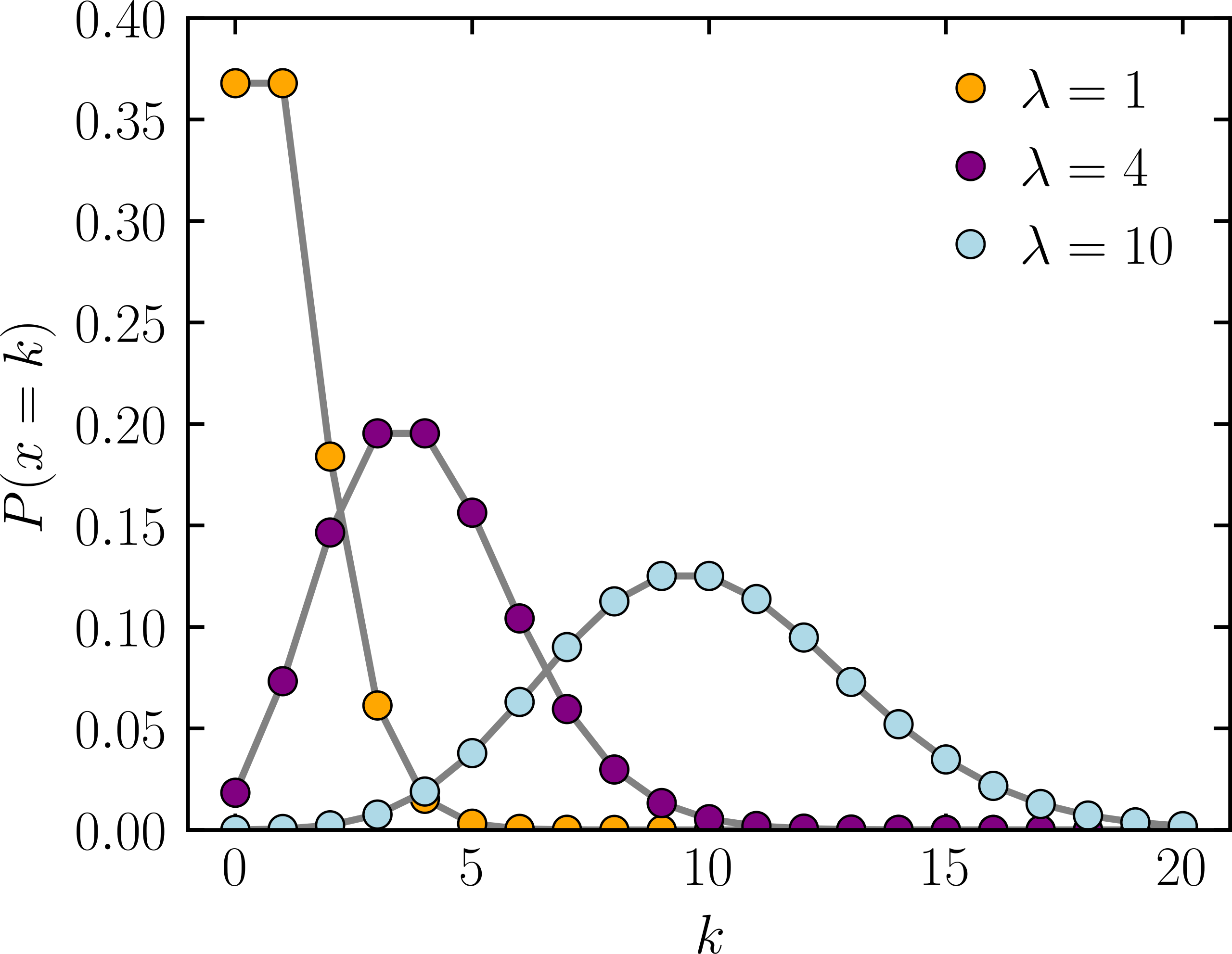
is the number of photons detected, is ... what?
Systematic noise from:
- Bias level - like ISO. Applied before the A/D converter to ensure the read noise is interpretable. Since the received photons will usually follow a Poisson distribution and look like a Gaussian curve, we "shift it" to avoid below-zero counts - corrected for with bias frames.
- Dark current - originates from the camera's electrical construction itself, from the random generation of electrons and holes within the depletion region of the camera itself - corrected for with dark frames.
- Multiplicative noise - non-uniform illumination, other sources, hot pixels, etc (often called "fixed pattern noise") - removed by using flat frames.
Characterization
We can characterize the noise and linearity of detectors using Photon-Transfer-Curves (PTCs):
Time
Definitions:
- Solar time: noon is defined as when the sun crossed the meridian.
- Mean solar time: allows each day to have the same length.
- In 1884, London decreed the Mean Solar Time would become Greenwich Mean Time (GMT) ... which then became UTC.
- ... which was then modified to become independent from GMT, now known as UT, as the time when stars cross the meridian (transit).
- UT Has versions - UT1 is most popular, UT0 or UT2 are also used (rarely).
- Standard stars used to determine UT.
- Transit telescope: slews along the meridian (north / south) to tell when a star moves across - does not slew east-west.
- Julian date: count of days since noon on January 1, 4713 BC.
- Created in 1582 by Joseph Scaliger to help make history line up.
- Synchronized with UT (i.e. J2000 is Julian 2000 w.r.t UT)
- MJD is Modified Julian Date - first 2,400,000.5 days subtracted to make the number shorter.
- i.e. measured since 1857 CE rather than 4713 BCE.
Days:
Sidereal (or stellar days) are measured with respect to the stars. Solar days are measured with respect to the sun - slightly longer because the Earth moves approximately 1 degree around it's orbit.
LST and Hour Angle
Local Sidereal Time (LST) and Hour Angle are the way we navigate using equatorial coordinates.
Spectrographs
Spectrographs:
- Take light from a source (into the telescope)
- Pass it through a slit
- Collimate it (force all beams to pass in a single direction)
- Push it through a dispersing element (like a prism to separate it)
- Pass it through a camera (to reform it)
- Send to the observer
Diffraction gratings are often used as the dispersing element (in place of a prism) because prisms can get really expensive.
Sometimes, folks will sandwich prisms, gratings and another prism, to form a GRISM - this is the case at APO's KOSMOS.
Taking spectra
We don't need great seeing for spectra - so they can be useful to take on nights with low seeing. However, spectra require long exposure times for reasonable S/N ratio in every pixel.
Guiding can be done by a "slit view" camera (i.e. spectrograph in center, normal otherwise) or via an off-axis guider (like at MRO).
Resolving power
For spectra, resolution is defined as
which can be for high-resolution spectra. is generally limited by slit-width.
Resolution can also be related to Doppler shift via
Wavelength calibration
- Find a lamp spectrum (i.e. using a dome light)
- Extract an ID spectrum using the same aperture and trace
- Using known lines and their pixel values, determine a dispersion solution
- Apply it to the 1-D spectrum
Checklist
Arrival
-
Log the level of the water tank. The water tank is located down the stairs heading toward the bedrooms, in the utility room on the right. The light to this room is (most inconveniently!) located on the left side of the doorway. Measure the water level by opening the valve to the gauge marked "in. H2O", which is located just above the water pump. The clear tubing will also match the level in the tank.
- Measure each day - refill if under 1/4 full.
- Prepare the water system.
- Turn on the water pump with circuit breaker 8 on panel M.
- Flush both toilets, which helps avoid the dreaded sewer backup!
-
Check the level of the water tank on a daily basis so as to avoid the (also dreaded) low water alarm.
- Do not turn on the water heater.
-
Prepare heat and air conditioning.
- If heat is needed - flip switch from 'Off' to 'Heat' on per-room basis.
- If AC needed, uncover the vents outside just north of the main entrance and turn on the AC circuit breaker.
- Add potable water to foot pump - in kitchen, put the kitchen tube in one of the big blue water tanks.
-
Initialize camera - on Sleipnir the Slow, open Evora (
http://localhost/on Sleip, orhttp://72.233.250.83/elsewhere on the network).- Initialize and set temperature to -82° C.
See Telescope Setup & Calibration for information on preparing the telescope for observation.
Departure
- Put away all media items (books, games, cables) in living room & observing room.
-
Kitchen:
- Wash dishes & clean up kitchen - wipe the sink down too.
- Collect trash & recycling to bring back.
- Refill kitchen and restroom soap dispensers w/ big soap bottle (add water if foaming dispenser).
- Restrooms - clean restrooms, wash toilets & sinks, sweep the floors.
- Cleaning the floors - vacuum floor upstairs, sweep floor downstairs.
-
Water cleanup:
- Measure water level and log it in the Google Doc.
- Remove tube from water jug under sink & seal it.
- Electricity:
- Turn off water pump circuit breaker.
- Unplug appliances & turn off power strips (don't turn off observing room computers).
- Turn off lights.
- Turn all thermostats off.
- Groceries - take pictures of inventories - note anything the next group should pick up from the store.
- Water jugs - put empty blue water jugs and empty clear plastic gallon jugs (if you can fit them) in car.
- Finalization - close living room shutters & all interior doors, and lock them.
This guide is shortened from the official version, available at https://sites.google.com/a/uw.edu/mro/checklist.
Telescope Setup & Calibration
- Initialize camera - on Sleipnir the Slow, open Evora (
http://localhost/on Sleip, orhttp://72.233.250.83/elsewhere on the network).- Initialize and set temperature to -82° C.
- Press 'Home' on the filter wheel.
- Initialize telescope - open Bifrost on Heimdall.
- 'Initialize telescope systems'
-
Make sure control paddle is set to
setnotslew -
Turn telescope on with key on RA skirt in dome
- Confirm 4 green lights in / around mount
-
Slew to zenith - use bubble level and hand paddle to bring scope to zenith.
- 'Load Zenith Coordinates' on Bifrost once this is done, then 'Update Telescope Coordinates'
Wait till sunset now.
-
Open dome
- Unclip dome power cables
- Plug in 3-prong lower shutter door motor, and round upper-shutter motor cable (note the upper-shutter cable has a specific orientation to follow).
- Raise upper shutter until the lower shutter motor turns on. Continue raising upper shutter, but you can now open the lower shutter.
- Once both are fully open, re-clip power cables where they were.
-
Remove telescope covers
- Make sure telescope is at zenith with correct RA/DEC in Bifrost
- 'Slew to Cover Position' in Bifrost - watch telescope cables. Emergency stop if it looks like anything's going to get caught.
- Use the ladder to remove the main telescope cover & the 6" finder cover. Store both on south table.
-
Take bias exposure
- It should look similar to this example bias.
-
Take twilight flats
- Move the telescope ~20 degrees east of zenith (west for morning flats)
-
Calibrate pointing
- Load
pointing_stars.txtin Bifrost and select a bright start with a low airmass. - Turn on tracking, slew to the star and then try to center the star in the finderscope manually with the Xbox remote. Click 'Update Pointing to Target' once it's lined up.
- Check another bright star nearby to be sure. Fine-tune to get to center-ish of FoV.
- Load
-
Calibrate focus - use a dimmer star for this one
- Goal is to minimize star PSF. Use focus helper in Evora for this - large leaps in focus increments on Bifrost are okay.
- Remember: focus is a relative measurement on the telescope, not absolute - "zero" focus is physically wherever the focus was when Bifrost booted up.
End-of-night
If dome flats needed: close dome, turn on dome flat light and point telescope at a relatively matte / flat area. Take flats as needed, then follow procedure below.
- Shutdown Evora.
-
Attach covers
- 'Slew to Cover Position' in Bifrost, then replace covers. Pay attention to cables.
- 'Park Telescope' to slew back to zenith
- Turn off the telescope with the key, then close Bifrost.
-
Close dome
- Rotate dome so cables are near ports
- Plug cables in - close smaller shutter (3-prong plug) first, followed by upper shutter
- After dome is closed, unplug and reclip cables.
Calibration Frames
| Frame type | Details | Exptime | Num | Periodicity |
|---|---|---|---|---|
| Bias | Readout noise on CCD - 'static' you see on low exposure times. | 0 | 50-100 | Few weeks |
| Flat | Help mitigate effect of dust and lens vingetting on lights - also acts as per-pixel correction factor. | 1-50 | ~50 | Every run |
| Dark | Try to capture noise from temp and ISO over length of exposure time. | LIGHTs | At least 5, ~20/exp | Every new exp |
Filter notes:
- Bias frames are filter-irrelevant.
- Flat frames are filter-specific - 1 every 5 exptime steps should work.
- Rerun darks every once in a while - build a library with ISO, temp and exptime.
- For sky flats, take them when sky is as bright (twilight) as possible with least sensitive filter, tracking on, with some offset between each exposure ... OR ... no tracking and allow startrails.
- Allows for variations in star intensities (i.e. frame 1 has a bright star, frame 2 only dark stars)
Telescope notes:
Bifrostdoes NOT record airmass in FITs header ... nor UTC or RA or DEC.- The MRO telescope will start to create "footballs" at ~12-15 minutes due to imperfect tracking - we could better this with a "real" pointing module.
Resources & Info
Resources, links and reference information for Manastash Ridge Observatory.
Location: 46.9511°N 120.7245°W
Resources
Evora Client - frontend website for controlling the MRO CCD camera.
Evora Server - backend to work with the Andor SDK 2.
Git cheat sheet - really lovely design, covers most use cases
Exoplanet transit calculator (NASA) <-- this should automatically set up for MRO
Exoplanet transit calculator (TESS)
Camera Info
The CCD is an Oxford Instruments Andor iKon-M 934.
Links
Fri. May 24 - Sat. May 25
José, Dylan, Eliz, Parker, Matt, Yasin, Ishan
Arrival
Acquired copious amounts of soda from Fred Meyer due to a bizarre buy-two-get-three deal. Arrived at MRO around 7:00 PM, skies clearing up from earlier rain, mid-50s temperature - hoping for clear skies tonight.
Checklist notes: Water level in tank after turning on the pump at 20% - refill next time.
Night - Fri. May 24
Notes:
- Always use the target list to start slewing. Make sure telescope is able to slew from Vega to Arcturus.
- Started the night aligning the finder scope with the 0.8m.
- Started observations around 3:30 AM - see problems log below.
- Nonlabeled flats are sky flats - domeflats are indicated such in header
- Wrote bash script to take domeflats automatically
| Object | Exptime | Filter | File | Notes |
|---|---|---|---|---|
| M57 | 10 | V | ecam-81 | |
| M57 | 50 | Ha | ecam-82 | |
| M57 | 30 | B | ecam-83 | DUST |
| M57 | 10 | B | ecam-84 | DUST :( |
| GJ 1243 | 35 | r | ecam-(85:105) |
Problems:
- Focus issues early on that we worked on until midnight - emergency stop of Bifrost software meant we lost track of current focus position. Eventually reset.
- Slewing / connection issues with Bifrost
- DUST - see ecam-83
- Same dust particles different filters? ... filter may not have moved or dust on CCDs.
Sat. May 25 - Day
Forgot to disable tracking while doing domeflats - telescope slewed entire night. Spent morning re-acquiring domeflats.
Pulled off CCD to see if dust effects were on it.
| Dusty darling | Better |
|---|---|
 |  |
 |  |
Wish List
Resupply
- AA batteries
- Recycling bin
- Sponges 🙏
Projects
-
Web interface to interface with both
evora-serverandBifrost- Dome control in web interface
- Weather details + webcam in web interface
- Autofocus mechanism - APO-style
-
Multi-filter series exposure planning
- Bash script already set up
- Old raspberry pi w/ wifi to act as an audio server (bluetooth and airplay, spot maybe)
Fri. June 21 - Sat. June 22
Oliver, Carter, Bruce, Maggie, Daniel, Thomas, Ruby, Parker, Anika
ASTR 481 Trip - Orientation
Fri. June 21
Arrived to observatory around 3:30 PM - after tour we made (slightly undercooked :( ) baked potatoes on the grill as well as beans / guac - ended up acceptably tasty.
Set up audio server to allow AirPlay, Spotify Play and Bluetooth - see below.
Around 11:00 PM started observatory setup.
- Sleipnir didn't boot for a long time - see details below.
- After Sleipnir woke up, we ran into issues with
telescopepinot starting - the mountedtelescopepiis a Pi 2 with an old version of the filter control software. The new version did not work withevora-server. Fixed corrupted Pi 2 with the old filter control software + restarted, no troubles after.- Old filter control vs. new?
Acquired Vega and Arcturus, until clouds moved in making further observation difficult. Trip snoozed around 3 AM.
Grocery List
- Out of white sugar, almost out of brown sugar
- Ginger powder as a spice
- Paper towels
- Aluminum foil
- Coffee creamer
- Plastic forks, napkins, paper plate
Inventory
 |  |
|---|---|
 |  |
Sleipnir
Sleipnir was acting slower than usual - ironically named. Boot hung up on something to do with SGX - apparently okay to ignore, but boot logs also showed some issue with an md5sum failed verification on a portable disk image (paraphrased). StackExchange answers claimed it was probably something to do with Mint, no solutions provided. Booting takes ~3 minutes as a result, in addition to the slowness of ubuntu.
To test whether the bottleneck was software or hardware, installed another distro alongside ubuntu - shrunk ubuntu disk 100 gigabytes and installed manjaro on it. Note - boot drive backup made at /home/mrouser/.backup just in case.
Results: Manjaro booted much faster, but still some of the same slow speeds persisted, even with no services running - so I bet it's hardware. Hard drive is a Toshiba MQ01ACF050 - 7200 rpm, Pentium 4 processor.
Audio Server
Set up an audio server connected to the 3.5mm jack on the vinyl-amp-thing - it supports connections via Bluetooth, AirPlay and Spotify Play, and can be further configured at http://audio.
As it runs on a Raspberry Pi, make sure the little black box with the fan is powered on and shows a red / green lights - if you run into any issues just restart it.
Thurs. Jul 11 - Mon. Jul 15
José, Naim, Parker, Ryan, Anika, Daniel
ASTR 481 Trip - Team 3 Trip 1
Week Goal(s)
Characterize Evora, the iKon-M 934 camera that MRO uses as a CCD imaging camera, by obtaining extinction and transformation coefficients.
While here, our plan is:
-
At the start of each observing run, take 10 bias frames to act as "per-night calibration frames".
- Thurs. 11
- Fri. 12
- Sat. 13
- Sun. 14
-
Create a set of <20 dome flats to find the shortest accurate shutter speed without seeing the remnants of the shutter.
- Done Sat. 13
-
Create a set of <15 sky flats to show linearity from minimum to CCD saturation.
- Done Sat. 13
-
Take a few darks to estimate Evora's dark current in counts / min.
- Done Fri. 12 & Sat. 13
-
Take 5 dome flats in and filters at around 80% of the point that nonlinearity begins (around 40,000?)
- Done Sat. 13
-
Take 5 sky flats in and filters around 80% of the nonlinearity point (similar to dome flats)
- Done Sat. 13
-
Observe an extinction star field over the course of several airmasses
- Thurs. 11 & Fri. 12
-
Observe standard stars at the lowest possible airmass
- Done Fri. 12
... and to observe some DSOs of interest.
Possible Interesting Objects
| Veil Nebula | Iris Nebula | Eagle Nebula | North American Nebula | Ring Nebula | Dumbbell Nebula | |
|---|---|---|---|---|---|---|
| Alt. Name | NGC 6960 | NGC 7023 | M16 | NGC 7000 | M57 | M27 |
Thurs. June 11
Stopped by Uwijimaya and Fred Meyer along the way to collect supplies for 5 nights' stay. It's nice out today - the skies are clear, temperatures high 70s. No bugs onsight in the observatory which was a welcome change. Started our epic dinner saga off by making sushi rolls!

After sunset, we started by calibrating the telescope. An issue that came up early in the night was that, for some reason after updating pointing to a target (i.e. once we got lined up with Vega), the telescope would stop tracking (without indicating such on Bifrost). This was resolved by just stopping and starting tracking again - still, curious.
Spent a few hours focusing the telescope and making sure it was pointing alright. Spent the remainder of the night taking pictures of GD 336.
Fri. June 12
Quiet day today. Folks started waking up around noon - we added the spare darkroom monitor to the observing room to try getting some more real-estate on Sleipnir.
Garlic brown butter tilapia for dinner - Ryan made some rice and Anika a salad to accompany our meal. Observations started tonight with little fuss - we continued with our extinction field GD 336 initially, then stars in our standard field SA38.
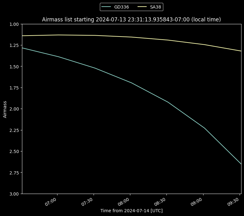
We noticed around 2:00 AM that the red lights in the dome might've been visible in the images themselves (tested with on and off) - decided to keep them on since they'd been on for the whole night thus far. More testing needed.
 Left: SA38 with lights on. Right: SA38 with lights off.
To end the night, grabbed some pictures of the Dumbbell Nebula (M27) and the Ring Nebula (M57).
Sat. Jul 13
Waffles for breakfast - started a Smash Bros Subspace Emissary campaign today within which we led a campaign of carnage (on normal mode).
Later, using SIRIL, I processed our pictures of M57 in false color ( to red, to blue and to green):
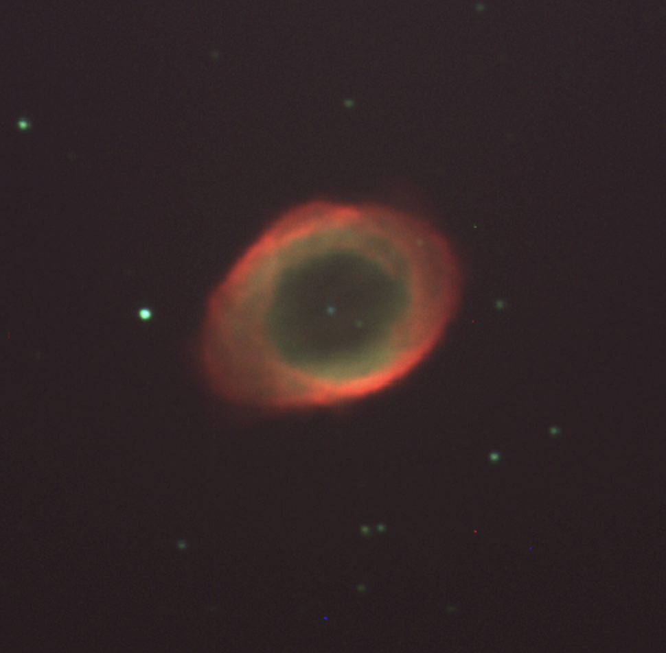
And the dumbbell nebula using a similar process
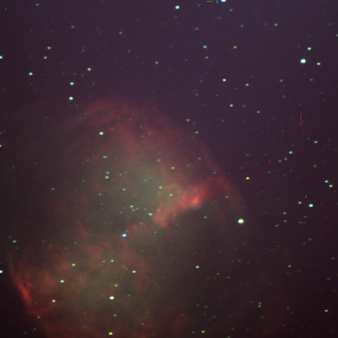
We hadn't applied our calibration frames yet, so I wonder how different they'd look if we did - let's try it once we get the master frames set up. Also each of these was only a combination of the 3 exposures - I wonder if we did a whole bunch of exposures whether we'd get a much higher SNR.
Wishlist item: a non-relative focusing mechanism. The focus seems to "drift" overnight and it can be hard to know when we're on target.
At sunset, we took our sky flats, then some dome flats and darks to finish up our first project report. Since we still had an hour or so until astronomical twilight, we tried training the telescope on the Moon - and saw this!
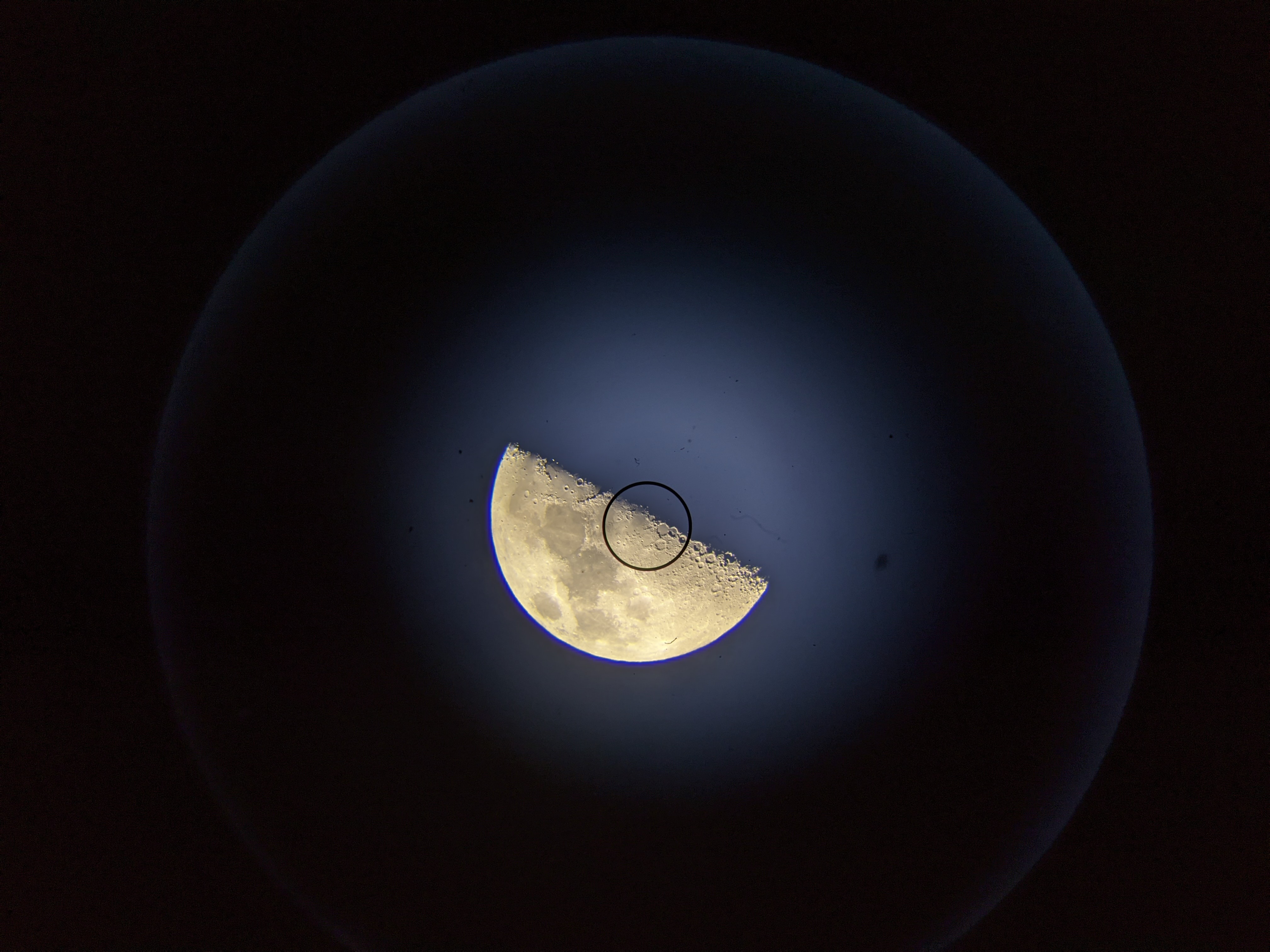
Since the Evora control software was modified to allow <1s exposure times, we were able to take ~0.3s exposures of the lunar surface.
After this, we sat down and watched the first Alien (1979).
Fun fact, the actor who played Bilbo Baggins in the Lord of the Rings (Ian Holm) was the same who played the science officer, Ash.
Sun. Jul 14
Cinnamon rolls in the AM, then more Brawl. Swamp is a hard level. Cleaned up some in the afternoon, then went on a hike in the evening. I think it was called Umpdenum Falls? When we returned, Ryan made some hotdogs with pickled onion - everyone was famished, so the meal was extra good.
Tried to take a look at some variable stars that needed observation on AAVSO, but we chose one that was a bit too dim (mag 16) to be distinguished easily - it was visible with a ~200 second exposure, but the SNR was so high that it was almost indistinct - so we packed it in for the evening, anticipating an early day on Monday.
Mon. Jul 15
Hoping to return to Seattle with some time to spare, we woke up around 8:00 AM and started cleaning, grabbing breakfast while we ran around getting everything back in order.
Inventory notes made in the class Doc and checklist followed, we packed our gear up and headed out around 8:45 AM, grabbing coffee in Ellensburg on the way back from Jenikka's.